1 Introduction
[hide]
This primer was written for version 1 of the script although it remains highly relevant to version 2 as well. However, the newer version does add additional functionality which is described in outline in Section 5. A more detailed explanation of the new functionality and how it may be used is available via video tutorials that can be accessed from within the script.
The Generalised Hyperbolic Stretch (GHS) Script offers a mathematically rigorous, yet natural way to stretch image data from linear to non-linear in a manner that allows for the flexibility to customize the results specific to the image properties, ultimate image utility and processor desires. By focusing the initial stretch on the data of interest, one can rapidly create a non-linear image that smoothly transitions between background and nebulosity, highlights the details of the subject matter, and retains the natural look of the brightest stars. In addition to the initial stretch, the flexibility of the script allows for either course or fine adjustment of the global distribution of brightness and contrast on already stretched images and even the repair of previously poorly stretched images. You can use the script for mask generation, colour saturation and balancing, or a multitude of other purposes currently only limited by the user's imagination.
Getting to the optimal use of the GHS script is admittedly a bit of a learning curve, but that doesn't mean it is limited to experienced Pixinsight users. Rather, it is the opposite, the GHS script provides a environment where good stretches can be performed on any images while the nuances of image stretching can be readily learned through trial and error. It is the goal of this script to get you started on this learning curve, regardless of your astrophotographic experience.
The largest part of this learning curve consists of understanding the nature of linear to non-linear transformations, how they appear on a graph, histogram and ultimately how they will make the image appear. It is hoped that this primer will get you started, but this learning curve takes practice and experience. This primer is long, and is deliberately geared to those who learn by reading. If you like to learn through experience, using a more tactile approach, then only give this primer a quick skim at first - take the script for a spin as it were.
Here is all you may need to know if you prefer to learn on your own...
- 1) You have the ability to design the stretch using 5 primary parameters while watching the histogram and previewing the results within the script itself
- 2) The D parameter controls the amount of stretch that will result in both a shift in the histogram and a widening of the histogram
- 3) The b parameter controls how focused the stretch is, how much stretch versus how much shift. Large positive values of b will bias the transform to image stretching or histogram widening in a highly focussed manner such as required during initial stretches of linear images. Large negative value of b will bias the stretch towards image brightening/dimming histogram. Fine adjustments can be performed with any b where b determines how "surgical" the adjustment is
- 4) The SP (symmetry point or stretch focus point) point places the focal point of the widening, shifting and contrast distribution. By default, the stretch or widing will be undertaken symmetrically about SP to account for where in the dynamic range of the additional contrast should be placed. While b is the stretch focuser, SP provides the place to put that focus. It's the SP, "S-point that places the S curve.
- 5) Two parameter LP and HP have two purposes. Firstly they are meant to preserve contrast (or protect) contrast within the histogram extremes. The second is they allow for assymetric stretches to be performed when used in conjunction with the other stretch parameters The scope and impact of these parameters will depend on how close to SP they are placed.
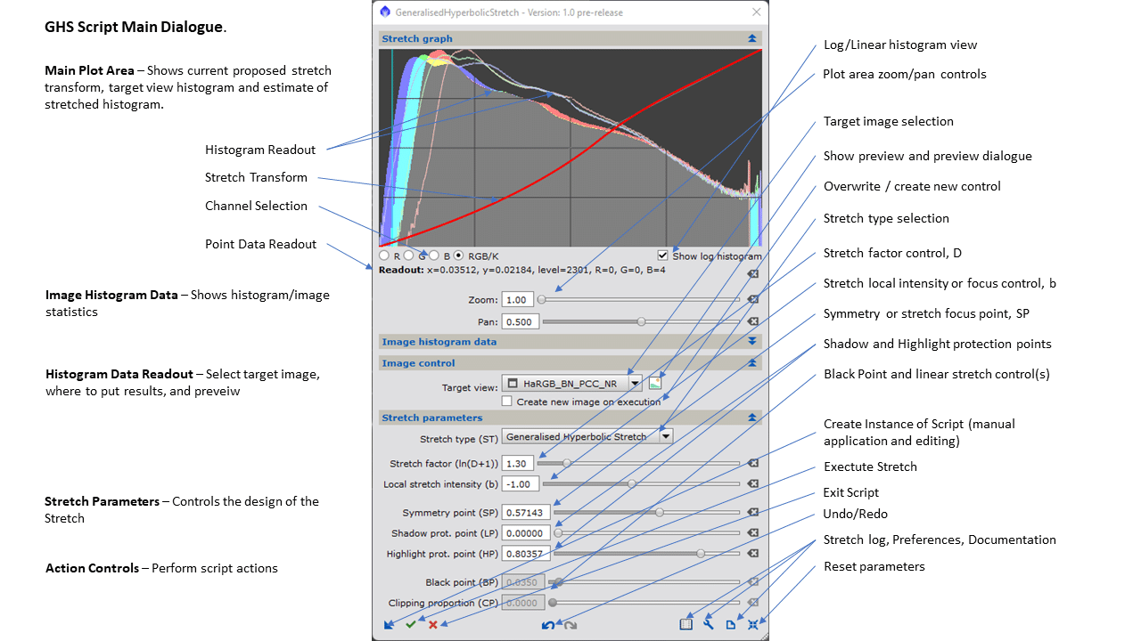
Dialog Controls are shown in Figure 1. Tool tips can be found by hovering over the controls.
If this works for you, great! You may still find the primer useful, as I have tried to include my discoveries and how to improve image stretches and perhaps they can be added to your own discoveries.
If you struggle to use it, don't give up, it took me a little while; although I was a co-developer of it, it was new to me at first too. I have tried to outline a systematic methodology to the use of the script that I believe will help. I have provided the information necessary to interpret the transform plot together with the histogram and image displays so that you can approach a stretch with a fundamental understanding of what to do and how to do it. Don't be intimidated by the math at all, I have provided descriptions of what they do to your histogram and image so they take on a functional character.
Remember there is nothing wrong with trial and error too! This is my favourite way of learning, especially when the errors don't cost anything other than time (provided you save your work and make clones). I have tried to include my own hints to improving the stretching process. However, that is not to say your methodologies might be better than mine or you have suggestions that I haven't thought of. The author bears no claim to be an expert in astrophotography himself. What I do bring is a great familiarity with applied mathematics in general, I have used this family of transforms elsewhere, and found a new application for an old solution.
While conducting stretches on my own images, I found I was either using one of two kinds of stretching tools. On the one hand, there is the straight up, rigid formulation that was pre-designed to quickly and easily (yet restrictively) get me through the stretching process with essentially one parameter controlling the amount of stretch, (D equivalent) that was "guaranteed" to provide me with a reasonable, yet often suboptimal result. The other type of tool allows me unlimited (artistic) freedom to draw any stretch curve I wanted, whether it would generate a reasonable result or not. Using this type of tool, getting the result a wanted ended up being a happy accident. I didn't really know why the result was good, or not, nor how to systematically reproduce, improve or duplicate good results.
When using the latter method on my own images, I eventually found that I was getting the best results when the stretch transforms took on one the forms of the generalised hyperbolic functions I was so used to using in engineering and science to forecast time series. To me, it was only natural to put these equations into a stretch transform that would meet somewhere in the middle of the two approaches - freedom to manipulate the stretch using more than one single parameter, yet having the restrictions to avoid doing strange things to the data or creatiing unwanted artifacts. It also provides a compromise between honouring the data, yet artistic freedom to communicate in a customizable way.
The next section is designed to walk you through the performance of an initial large stretch(es) of a linear image to get you most of the way to your final stretch. During this walkthrough, the primer will describe how the stretch works, a more detailed description of the stretch parameters, and the many features of the script that allow for the design, preview, and execution of the stretch itself (thanks Mike!). Section 3 completes the description of all the input parameters, explains how to refine and edit your stretch, shows some of my tricks and tips, and how to integrate this script into your Pixinsight workflow.
Completeness and curiousity were the only drivers to include Section 4, where the equations are described. You can skip this sections entirely if you like, but it's here if you either need or are curious as to where the transform equations come from. Suffice to say that they have been selected from a family of occuring curves (Generalised Hyperbolic Equations) found throughout science, nature, and even economics, often used for analytical or empircal modelling and forecasting of time series functions, such as nuclear and chemical reactions, epidemiological modelling, oil/water/gas well production forecasting, and even compound interest calculations.
This script is brand-new as of writing this primer, so I am sure I am leaving a lot out despite the length of the primer. Please post any omissions or shortcomings you see so that the functionality of the script itself can be expanded or modified. Also, please provide any additional tips or tricks so that they can be included in this primer.
I have only started to use the script and have already enjoyed a step-change in the quality of my own images. I hope you have the same experience with yours. I also hope that, after an initial struggle, you will find the script easy to use and it becomes "second nature" as it is becoming to me. Even if you decide to not use the script, we believe that following along with use may provide some insights on the image "stretching" process, ie. going from linear images to non-linear.
While the original conception was mine, the true brainpower behind the script is it's author, Mike Cranfield and I would like to acknowledge his skill and effort in bringing the script together.
2 GHS Script Walkthrough - From Linear to Non-Linear
[hide]
In this walkthrough, we will attempt to introduce you to the script environment and its facilities, how to interpret, control and design a stretch function, and how to successfully make an initial stretch an image in 1 to 3 steps. In getting there we will be taking an almost painfully methodical approach to interpreting the image, the histogram, and the stretch transformation itself to see how you can use these tools in tandem to perform an initial stretch where you can't actually see what you get until you get there. Please follow along with your own image because, by doing so, I believe you will get the most out of it.
At first, we will try to stretch a image using only the single "stretch amount, D" parameter and the default, exponentential (b=0) form the of the stretch equation. By using only this parameter, I can almost guaratee you that this won't be the best stretch you can perform. Fear not, however, as this is only being used as an example and a route to showing how we can custom design a stretch for your image
- interpret the stretch function graph in both brightness and contrast terms towards understanding how to tailor a stretch function to the image itself and to the desired results.
- how to interpret and use the histogram to guide the stretching transform
- how the individual input parameters change and control the input transform. Included is an introduction to two additional transform parameters that will greatly improve on your initial stretch. Together with the preview and histogram, you will see how to use these parameters in concert to get the best, custom stretch
- how to use the display, preview and inquire the stretch, to further hone in on the best set of parameters and stretching sequence
Trust that once you get the "knack" of what the script and the stretch equations are doing, the process can be very straightforward and quick. Also, please take my opinions on "what should be done" with a grain of salt. These are only my opinions and you are, of course free to try whatever you like - there are an infinite number of ways to employ the equations and stretch, only a fraction of which have been undertaken by this author.
It is assumed that you are familiar with downloading the script from your source, and getting Pixinsight to recognize the script within it's pull down menu using the "Feature Script" utility. If not, there are plenty of resouces available to help you with that within the internet and it is beyond the scope of this primer.
2.1 Starting the GHS Script
The use of this primer and the GHS script itself are best used by following along with an example. The best example would be of a linear, well calibrated stacked image that has previously undergone all of the linear processes that are parts of your normal workflow, i.e. ready to be stretched and made non-linear. My normal practice is to save the image at this stage, and start the script using a clone of this file. It is helpful if you have a sense of the distribution of pixels, gained by examination using the STF of the image. Helpful information also includes, what portion of the image is background, what portion is stars, and what portion occupies the principle subject matter of the image (nebulosity, galaxies, star clusters). In the unstretched, linear image, are the stars nearly saturated or clipped? Are there stars throughout the brightness scale? Is the nebulosity distinct from the background or does it fade into the background? It is important that the target image be available as a view or icon in the current workspace (ie. is actually an open image).
Note that certain image processing processes work best, or even require, that the input image is linear (eg. deconvolution), so you may want to ensure you have conducted all your desired "linear" transforms prior to using the script. In addition, it is also often beneficial that some noise reduction be performed prior to use of the GHS script. Some stretch transformations may result in the exaggeration of the noise, making the result appear even noisier and making post-stretch noise reduction very difficult.
If you are an experienced image processor, take a few moments to see what you like and don’t like about the STF stretch. Are dim features visible? Has noise been stretched also? Is contrast in the image where it is supposed to be? Are the stars bloated? Has the colour saturation been lost? Has the contrast and dynamic range been applied where you like? Have features you would like to bring out being highlighted? Is the image the desired brightness? This script is meant to be customizable for your target image, and by customizing the stretch, you should be able to do “better” than the STF stretch itself so it is good to define what you feel would be “better”.
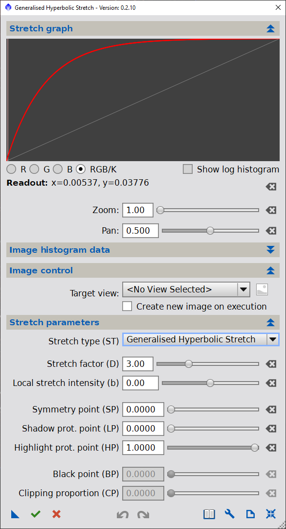
To get started, select script==>Utilities==>Generalised Hyperbolic Stretch. Upon start-up you will see the first image in Figure 2 (or something close.) representing the main control dialog screen for the script. The main dialog consists of four tabs/areas:
- a multi-purpose plot area used to display a graph of the current proposed transform, a histogram of the target image prestretch, and an estimate of the post-stretch histogram
- a hidden tab to show image and histogram statistics
- an area to select the target image for the stretch transformation, preview controls, and what is to become of the transformed image
- the controls for the stretch transformation itself
If you are following along with this walkthrough, then for now leave the target image unselected so that we can focus on plot area, the transformation graph and how to interpret it.
2.2 Interpreting the Stretch Plot Curve and the stretch factor "D"
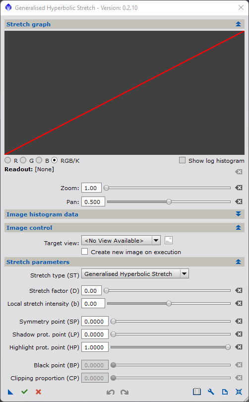
The plot area at the top of the screen has multiple purposes. Firstly it shows a plotof the transformation that the script is about to employ, analogous to the plots you may already be familiar with in the “Curves Transformation” (CT) process. Along the x axis is the brightness, intensity or input value of a given pixel in the proposed target image. Along the y axis will be the corresponding pixel value after the GHS transform is completed. Upon opening the GHS function is set to y=x, ie. the identity transform – or no stretching. As we will see, this y=x will be important.
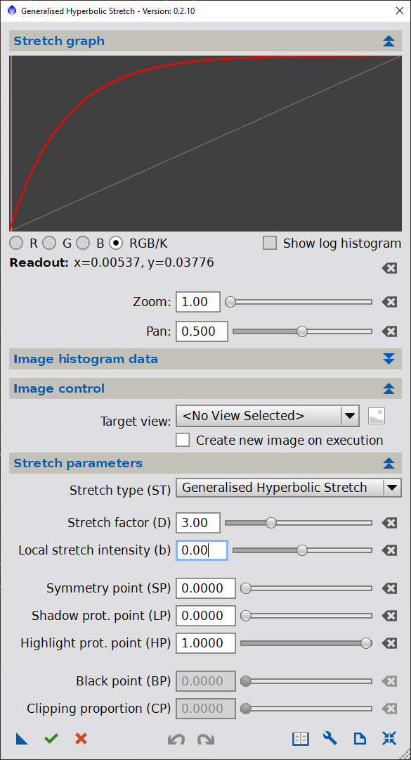
Within the image controls, you should see that the stretch factor (D) is set to 0. Regardless of the other parameters used to control the stretch transform, when D is set to 0, the identity transform, y=x, will be displayed. In this section of the walkthrough, we will be dealing only with this D parameter and how it control the magnitude of the stretch that the script will undertake.
Before proceeding, lets review how to interpret the transform plot. To start, move the stretch factor (D) “D” slider to the right to 1 or manually enter (type 1.0 into the text box and hit enter. Alternatively, mouse over the above image to the appropriate "Exponential Stretch D=1 value.
What you should see is the red line move to a curve that lies above the identity y=x line, which is still shown in the plot in grey for reference. The red curve itself represents the non-linear (in this case, an exponential curve) that indicates, for every x=pixel value, intensity, or brightness, what the resultant pixel value or brightness will be after application of the stretch (y value).
Note that the curve runs through both the points (x=0,y=0) and (x=1,y=1), such that pixels with an input value of 0 and 1 will remain unchanged. This is the case for any transform performed with the script. Since elsewhere, the curve always lies above the y=x, all the remaining pixels between x=0 and x=1 will be brightened to some degree, however, none of the pixels will be increased or "brightened" to a level of 1, except if x=1, because the curve only reaches a level of y=1, when x=1. This is true for all of the stretch functions that this script is able to apply. In this way, all brighter (or dimmer) pixels will still be brighter (or dimmer) in the resultant image - ie. the rank order of pixel brightness will be maintained.
Note also that each possible resultant y value corresponds to a single x (unstretched) value, meaning that the stretch represents a 1:1 mapping of pixel values. As a consequence there is (theoretically) no loss of data in the transformation (excluding digital resolution issues), and that the transformation is completely reversible, and repeatable. In plain speak, this means you can always recover data that is hidden in shadows or lost in brightness - even returning an image to its original linear state. This is a fundamental difference between this script, and application of the CT process. With the CT process, the user is free to violate this 1:1 mapping constraint, and in some circumstances it may even be desirable to do so. However, with the freedom that CT provides will come consequences regarding repeatability, reversibility data integrity, and artifact generation. The choice between this script and CT is yours to make, but understand that this restriction in the GHS was purposefully built into the script for reasons that should become apparent.
The stretch function can also be thought of as a redistribution of both brightness and contrast, within the constraints of the image file to record them - the screen, monitor, or paper to represent them, and our eyes to actually percieve them. It is useful to consider the stretch transformation graph in both of these ways: as a dynamic change of the image brightness and as a redistribution of contrast.
Ultimately brightness is constrained by the maximum brightness of a pixel (represented by x=1), and the total absense of pixel illumination represented by x=0. If we had pixels that were unconstrained in how bright they could get, we could brighten any image simply by multiply their values by a constant (eg. 2, or 10, or 100) stretch factor until the image overall stretch yeilded a comfortable brightness for viewing. This would be a linear stretch and would work marvelously (assuming our eyes percieved brightness linearly as well). However, our pixels are limited to the amount of lightness they can emit (from a monitor) or reflect (from paper), and if we applied such a linear stretch, we would find that any pixels brighter than x/C would be set at the brightest level possible and be clipped. We would not be able to distinguish between pixels that are "clipped" because they would all show the brightest or largest level possible. To avoid this, all stretching functions must compromise on this stretch factor.
On the plot, the actual stretch factor or multiplier (define by y/x) that will applied to a given pixel value is represented by how far away the curve lies from the y=x line. If you increase D above D=1, you will see that the stretch transformation curve gets further away from the y=x line, representing a larger stretch overall for the image. In fact, D is one of the main controls we have on the stetch function itself - if you want to stretch a dim image a lot, a high D should be chosen, of if you want to stretch an already bright image a little, then a small D should be selected.
The maximum stretch factor that will be applied to a given pixel lies somewhere in the middle of the pixel value range. For D=1 (leaving other parameters at defaults), this occurs at about x=0.4 or so. As D is increased the maximum stretch factor that is applied moves to the left, and at extremely high values of D, it approaches x=0 itself. The stretch function almost becomes blocky, and reaches close to its maximum value of y=1, just to the right of x=0. You can relax, however, because the function itself cannot achieve this result - and even though it appears to hug the LHS and top of the graph area, in actuality, it is retaining its functional shape (within rounding, or numerical precision error). You can check this by zooming in on the fuctions using the controls just below the plot itself.
You can verify through zooming that the plot transform only reaches the y=1 value at x=1 - using the zoom control just below the plot area. That doesn't mean that an image can't be over-stretched, it is just pixels won't be clipped. It is a goal of image stretching to impart the best amount of stretch factor to the right parts of the image so that the subject matter(s) within the image is displayed with the desired brightness.
It is also useful to think of the curve in terms of contrast redistribution. Contrast allows us to distinguish between and within subject matter in the image itself. Contrast distribution is yielded from the stretch transformation from the slope of the curve. Unfortunately, the amount of contrast a stretch function can impart to an image is also constrained. Since the stretch function must always go through the point (0,0) and (1,1), its average slope over the whole 0 to 1 range must be 1. That is, overall, the stretch functions can only take contrast away from part of the image and give it to another. Where the slope is greater than the y=x identity line, the stretch function is adding contrast, and where the slope is less than the identity line, contrast is being decreased. Unlike brightness, which is only constrained by the limits of display, there is only so much contrast to go around and employing a stretch transform must take from another portion of the image to give somewhere else.
Lets move through various values of D again, either with the script or the figure above to see where contrast is being redistributed to, this time looking at the slope or steepness of the stretch transform function throughout the x range. In all cases where D>0, you will see that the maximum slope of the curve occurs at x=0. Actually the slope at x=0 is set exactly to D! (note D entered into the slider value is actually the log of D as used by the script). The slope then declines towards the RHS. (In fact, it exponentially declines - imparting this name to the stretch function). It continues to decline at a rate (2nd derivative), inversely proportional to D, towards increasing x so that at x=1, it's actual decline is such that its average slope over the range of x reaches 1 at the same time as x reaches 1 and y reaches 1. In this way, the effect of increasing D is to shift maximum contrast to the increasingly dimmer parts of the plot area - to the LHS while taking it away from the brighter parts on the RHS.
Where contrast is placed is a matter of taste and the purpose of the image - which brings us to the second purpose of image stretching...It is also a goal of image stretching to impart the limited amount of contrast available to the right parts of the image so that the details of the subject matter are most observable to our eyes.
What we have been observing so far, is how a single parameter, the stretch factor "D" affects an exponential stretch. Such an exponential stretch is likely the simplest, most natural stretch to apply to an underexposed daylight image. The form of the function, in this case "exponential", actually defines the proportionality of brightness change and contrast redistribution. However, the characteristics of the astronomical images likely means that an exponential stretch is not necessarily, nor even likely, the best form of stretch to apply to astronomical images in general, let alone to a specific astro-image. After all, we have two defined goals already, to place contrast in the right places, and brighten the images the right amounts in the right places. This is a tough task to achieve with one form of the equation (exponential stretch) with one control parameter, D. Soon, we will encounter other parameters that will greatly expand this seeming limitation. Not only will we be able to change the amount of stretch D, but also the governing shape of the stretch function so we can control these relative proportions.
Some of the utilities within Pixinsight (including the arcsinh stretch (AS), and the Histogram transform (HT) / Screen Transfer Function (STF) itself propose general purpose formulations that work well for many astro-images. However, in the most successful images I have seen, the use of these tools are almost always followed up with one or more of the "Curves Transform" where hand-drawn transform functions are applied, interpolated with splines. While the CT process can get us away from the rigid "single function" limitation, it has potential pitfalls of its own. One of the goals of this script is to avoid the errors and time requirements of "hand placed" points by using well defined equations and specific parameters. In that way, the best of both worlds can be had. In the following sections, you will see that other parameters are available to achieve your desired results with almost limitless flexibility.
It should also become apparent that there is no "right" or "wrong" way to stretch an image. In fact, even within this script, there are many ways to achieve essentially the same thing. There are perhaps "better" and "not so great" ways to stretch an image, but even this is subject to the law of diminishing returns, and the point may be reached in stretching where you need to call enough is enough. Recognized the point that the GHS script is a global tool, and many tools, including HDRMT and LHE exist within pixinsight to locally change stretch and contrast and in no way can this tool displace this functionality.
What is helpful, however, if you can look at a stretch transform function and recognize what it is doing, where it is stretching, and where it is placing contrast. If it is a bit cloudy still for you, please move ahead with the following section and re-review this one later. Following along with the walkthrough should clear this up.
2.3 Using the Histogram to Define an Initial Proposed Stretch
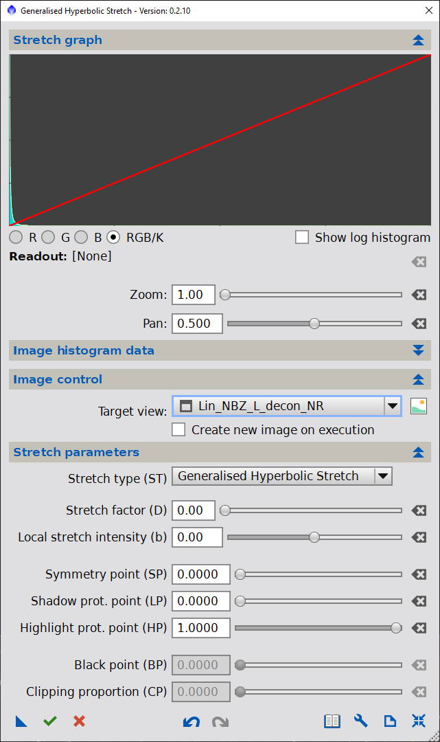
If you are using this document as a walk-through, then lets refresh the input, or move the D slider back to 0. Secondly, to view a histogram we need to load in an image. In the pull down in the image control section, select the image that you wish to use to follow along this walkthrough. Upon image selection, you may be asked if you would like the STF removed from the image. Answer yes to this question and your image view will be restored to its linear state. If there is a mask currently applied to the image, you may also be asked whether you want to remove this mask for stretching or leaving it in place. We will discuss masking in section 3 of this document.
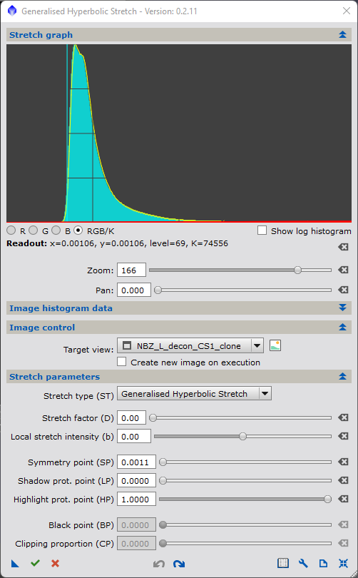
Upon selecting the target image, the script will display, in the same plot as the identity transform graph (because currently, D is set to 0) the histogram of the linear image. In general, this will appear as a occupying the left side of the histogram only, as shown for the target image that I loaded in the Figure 3. For your image, the histogram may appear more to the right if more exposed, or barely visible at all if less exposed. In actual fact, this histogram peak generally contains the majority of the pixels in the image - both the background and likely any nebulosity. On the image itself, you may only be able to see the centres of the brightest stars and while this is the only part of the image that is visible, it represents very few pixels on the actual image. Mouse into or click the first image of Figure 3 and note the histogram on the far LHS. It's likely difficult to discern anything about the linear image from this view.
The GHS script facilitates the examination of the linear image in two ways. Firstly, we can display the histogram in logarithmic form. If you are unfamiliar with this, it is the same histogram, only emphasising the view of "few" pixels while diminishing the impact of many pixels. If you click on the "show log histogram" check box, or mouse over the second image in Figure 2, you will see that there are at least some pixels of all values pretty much throughout the range of brightness. It is just that the vast majority of pixels are very dim and you can't see these brighter pixels on the linear version of the histogram. In many asto-images, these pixels over the majority of the histogram likely represent stars and small, brighter images. The log histogram view is particularly good at checking on the stars or brightest part of the image. If the log histogram pixels reach all the way to the right, then the brightest portions of the image have likely been somewhat overexposed and clipped by the dynamic range of the camera. This is ok to some degree for the brightest stars, but what we want to avoid is a significant second "histogram peak" to develop on the RHS - either through image exposure or through stretching. This will make stars appear large (bloated), or opaque, and unnatural.For our image, we see there is very little, if any, clipping of the linear image. Also, of significance, is whether or not deconvolution has been applied to the images (as has been done with the image in the example presented here). Deconvolution tends to make stars brighter than in the original image.
Where the stars exist in the histogram is important for stretching, however, because the bunching up of stars on the RHS of the histogram will make them appear bloated (excessively large, bright and artificial) and likely detract from the subject matter of the image itself. As stated above, the GHS script will maintain the rank order brightness of the pixels - ie if a pixel is brighter in the unstretched image, it will remain brighter in the stretched image. At the same time, our goal is to brighten the pixels at the LHS of the image - which will necessitate brightening the pixels on the RHS of the histogram, potentially causing the star/brightest pixels to "bunch up on the RHS. Additionally, we have seen that the base exponential stretch transform redistributes contrast by concentrating it at x=0 and at the same time, taking it away from the RHS (contrast = slope, and the slope is least on the RHS, greatest on the LHS). The combination of the two can leave the stars looking flat and bloated.
Next, lets look at the histogram more closely by using the controls below the plot area to zoom in on the histogram peak, that will likely be concentrated on the far left of the plot area, or mouse over the zoomed in histogram (third image) in Figure 2. This histogram peak likely contains the background pixels of the image and a lot of the nebulosity or foreground subject matter. In order to see the image properly our stretch will have to move this histogram to the right (ie. brighten it) and broaden (widen it) to be able to distinguish the background from the subject matter. How far to the left the histogram is, and how concentrated (how thin and peaky it is) will play a role in how you stretch, and ultimate how the image looks after the stretch. Moving the histogram to the right involves the stretch factor that is to be employed. Broadening or widening the histogram peak involves inserted contrast within that small histogram peak. Aside from the histogram width and peak, a third parameter to take note of is the size of any gap between the left side (x=0) and the background signal. If there is no gap, then the image is underexposed and you have not captured background (or have clipped in linear processing steps) some of the details. If there is a gap, then the width of this gap will determine the brightness level of the background.
While the focus of our initial stretch will be on the LHS histogram peak, it is alway important to note where the stars are in the histogram. Fortunately, there are a number of ways to protect the stars and even repair the stars within this script, as we will see later. In the meantime, you should endeavour to be aware of where the stars are in your histogram and what will happen to them in the stretch. Mousing back over the image in Figure 2 to show the logarithmic histogram, reveals a good distribution of stars brightness throughout the histogram without a lot of clipping, bloating, or flattening. Our challenge will be to largely keep it that way.
Now that we have examined the histogram, let's try out the stretch, using the histogram as a guide. Begin to move the D slider to the right keeping an eye on the how the histogram changes. If you are zoomed in on linear scale, you will start to see a "second" histogram appear overlain in the plot area. This second histogram is actually the transform applied to the original histogram using the current value of D, and is an excellent guide, if only approximate, as to where the stretched image histogram will end up. The more you move the D slider to the right, the more you will see the second histogram move off of the original and move to the right. If you are zoomed in, you may have to zoom out as the histogram shifts completely off to the right of the zoomed in view. Once you are zoomed out, for now, try and move the histogram such that its peak ends up at approximately 0.25, or one quarter of the way to the RHS. If can cannot reach this point with the transfromed histogram, simply leave the D slider all the way to the right. Do not execute the script yet (or if you do, please undo the execution) we have some other fish to fry first. As a rule of thumb (feel free to break it) you should place the histogram peak at a value of about 0.25 in your final image. THis is consistent with the STF function.
As an aside, to improve the utility of the D slider, the number entered is actually the natural logarithm of D. This is done so that very large values of D can be used in the stretch transform equations. This means that, at very large values of D, precision in specify a D may require input of the value of D into the text box of the slider. At lower values of D, however, the slider provides great accuracy on its own. You may find it necessary to manually enter D in this exercise, depending upon how precisely you wish to place the histogram peak. To get the actual value of D used by the equations, calculate this as exp(D)-1 from the slider.
If you are using a colour image, the plot area may become fairly busy with three colours, two histograms, and the transform function all shown simultaneously. This may appear confusing at first, but having all this information on a single plot area will help enormously later. In the meantime, the default setting are such that the original histogram appears only in outline, while the transformed histogram will appear solid. You can change these defaults in the preference dialogue of the script as shown in Figure 1. The example being shown in the Figures 3 is a monochrome luminance image extracted from a filtered one-shot colour (OSC) camera.
Let's now use the preview facility to see what we are proposing to do to the image itself.
2.4 Previewing the Image Stretch and Enquiring the Image itself
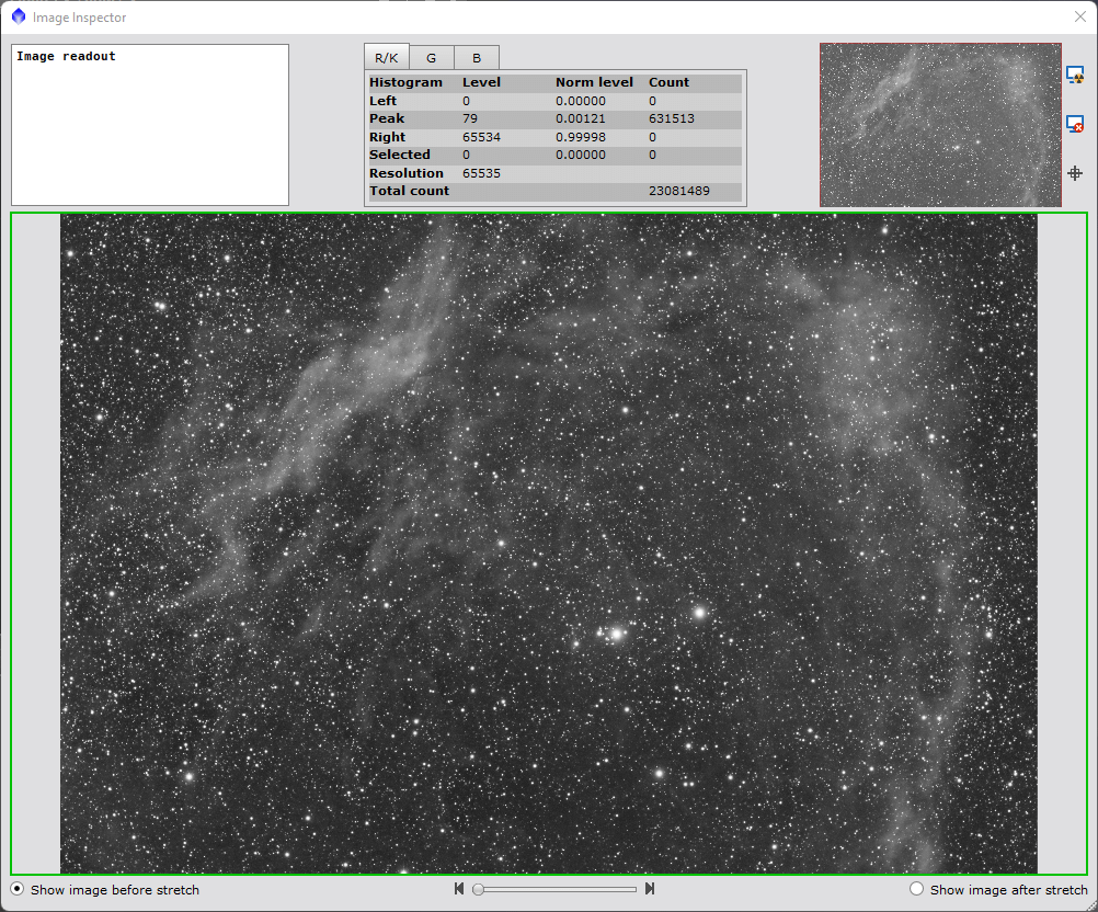
By clicking on the image icon next to the target view selection dropdown, a new dialog will appear, initially displaying a copy of the target image in its unstretched form. This new "preview" dialogue can be also be seen in Figure 4, below by mousing over/clicking on the first image listed (controls are shown in Figure 1). There are multiple purposes of this dialogue, but the two most important are enabling the enquiry of pixel values on the image iself, and enabling a preview prior to execution of the stretch itself.
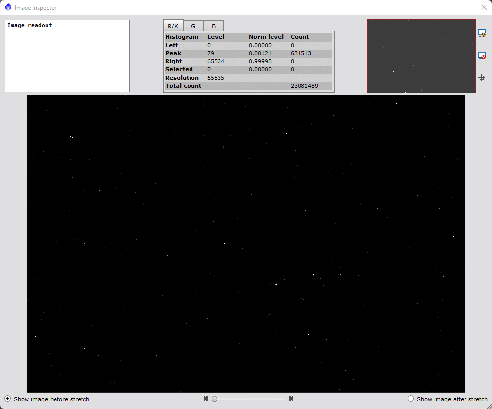
The first view one sees upon openinig is of the target image itself. As in our current case, the image is still in linear form, and you may only be able to the brightest stars in the image. When this is the case, you will likely want to perform an STF on the image again by hitting the familiar icon in the upper right portion of this new dialogue (see image 2, Figure 1). Note that the application of the STF is for image orientation purposes only, and is not attempting to display the results of the stretch transform being applied. At the same time, the STF view creates a "benchmark" for us to consider the current transform contemplated.
By clicking on the image area, the dialogue will display in the upper left, the current value of the pixel value, and the resultant pixel value from the proposed transform. The ability to enquire the pixel values from the image may not seem critical at this stage, but as your familiarity with the script increases, it will become very value in relating the image to the histogram on the main dialogue. If you click on a detail or feature you wish to either highlight (or hide) in your final image, you can determine where this point exists on the histogram, and then modify the histogram transform appropriately. The facility exists on this dialogue to also zoom in on the image to make more detailed inquiries.Note, when zoomed in, either the thumbnail in the upper right of the dialogue or click-dragging on the image itself can pan the zoomed in image.
Finally, this dialogue has the ability to perform the currently proposed transform on the target image in a preview manner by selecting the "Show image after stretch" button to see if the currently proposed transform produces what it desired from the stretch. On a base level, if you like it you can go back and apply and if you don't you can exit the preview, and make some adjustments and return. You can also compare what a simple STF/HT processes will produce versus using this script by comparing the STF applied to the original image, with the GHS transform by moving back and forth between the ustretched image, with STF applied to the preview of the image with the proposed stretch applied. (A convenient way to do this is by selecting <cntl+leftclick> on the image itself or <cmd-click> on a Mac). You can see this for my image by mousing over the the second and third images shown in Figure 3, which will show the unstreched STF image in the former, and the GHS applied in the latter. Note that if the proposed stretch does not fully brighten the image, an STF can applied to it to "see" what would become of the image should you apply a STF equivalent stretch the rest of the way.
Now, it is more than likely that you prefer the STF on the original image, better than the results of the currently proposed GHS stretch transform - certainly thats how I feel by comparing the second and third images in Figure 4. Here is why I fell that way:
- 1) While the stars are somewhat bloated in the STF image, they are considerably more so for the proposed stretch. This is also evident by looking at the proposed stretch histograms - you can see that the pixels have started to pile up, forming a peak on the RHS of the histogram - mouse over the fifth and sixth images in Figure 3
- 2) There is far less contrast (and brightness) in the nebulosity in the proposed stretch Nebulosity should be the star of the show, and while the brightest nebulosity can be seen, details in the dimmer nebulosity can't be seen
- 3) The background brightness is higher in the proposed stretch. This makes it very difficult to distinguish between dim nebulosity and background.
Several reasons are reponsible for this result all related to the differences between the STF function and our exponential stretch. Firstly, the STF transform is gentler on star stretch (protects the stars more) than a straight up exponential stretch as proposed using our current settings of the GHS script. Secondly, the stretch factor is focused more on low pixel values than the exponential stretch - resulting in greater brightness of some features hiding in the unstretched image. Thirdly, the background is brighter in the GHS image which may or may not be desireable, but it is automatically corrected for in the STF while such a correction is performed in a different manner, or as a separate step in the GHS script. Remember that the STF stretch itself, has been formulated to be and I believe succeeds as the best generic, all round stretch function that I have seen and really sets a good benchmark. The point here, is just to highlight some of the things that can go wrong with large stretches without considering the data itself and using only one parameter, D, to define the stretch function. In order to "beat" the benchmark, we will have to introduce a couple of additional inputs to the GHS stretch function.
If you are following along, close the preview dialogue screen to return to the main GHS dialogue.
2.5 Local Stretch Intensity, "b" using Base Equations (b>0),
Of the five parameters in the base GHS application, we have only explored the first, the Stretch Factor (D), to control the amount of stretch employed and we have used this to move a linear image's peak histogram location from it's linear location to a more visible point (at an intensity of 0.25), leaving defaults for the other four parameters. We have also looked at a preview of the results, perhaps determined what we like or dislike about it, including a comparison with the STF results. To proceed, lets take a step back and introduce a couple of more parameters for the GHS stretch and see how they can be used to improve our stretch. Hit the reset parameters on the main dialogue screen and deselect (for now) the target image (select "No View Selected" in the pull-down). Move the D slider to a value of about 3.5 (a moderate) stretch for illustrative purposes, and you should be able to duplicate the image on Figure 4.
To this point we have left the second parameter, b at b=0. As we have discussed, this means that the GHS transform represents an "exponential stretch". For the lack of a better label, we have called the second parameter the "Local stretch intensity" as on a certain level, that is exactly what it does. More fundamentally it changes the form of the transform itsef in a manner that needs explanation, but without too much effort, will become clearer as it is used. Let's start by move the b parameter to the right to about 0.3, illustrated by mousing the second selection in Figure 5, and then to b=0.6 and follow along observing what is happening in terms of both the stretch factor (height of the transform above y=x) and contrast (the slope of the transform). Technically, speaking, the mathematical form of the transform moves from "exponential" when b=0 to "hyperbolic" when 0<b<1.
In terms of the image transform, when b is increased, the nature of the transform and its imparted contrast (the slope of the transform) very close to the x=0 point remains unchanged. However, relative to the exponential curve, the slope begins to reduce earlier and more rapidly towards the middle of the plot area. Then somewhere in the middle, the stretch fact slows its reduction in slope and becomes increasingly linear (but doesn't reach linear) in form at high values or on the RHS. What this means for an image is that the stretch remains the same at x=0, increased near x=0, but it is reduced for the rest of the image. Ultimately, this change means that for a given input D factor, increasing b achieves greater protection for the stars, helping avoid "star bloat". It also moves the "maximum stretch factor" closer to 0, creating a more concentrated stretch near the zero point, while reducing the amount of stretch everywhere else. This trend seems to be exactly what we need, a more concentrated stretch where the nebulosity resides in our image, with a gentler stretch on the brighter (stars) parts.
You can aslo see the impact of raising b by mousing over the images in Figure 5.
In practice, when using an increasing b you will also likely increase D in tandem if you intend on "placing" the maximum histogram peak at a certain level. The net effect of increasing both b and D (to compensate) is that the stretch becomes more focused around x=0. For larger stretches in general you should select a larger b value, the more concentrated or skinny, the original histogram is.
Increase b to 1.0, and the stretch function becomes reaches a special form (next mouse over on Figure 4). At this point, mathematically the stretch becomes "harmonic" (ie. related to inverted intensity) and becomes a good general moderate to large stretch factor, balancing off stretch concentration one the LHS with star protection on the RHS of the histogram. Indeed, this form of the stretch is almost exactly the same as the STF / Histogram transform itself (harmonic) and is why the HT is so successful on its own - essentially requiring only one input (essentially "D" in another form) as its input. In fact, the HT process transform, (which also contains an inherent linear mask) is duplicated within this script (select "Histogram Transform" under "Stretch Type" if you wish to use the exact formulation within the GHS script). Using a larger b, at 1.0, or selecting the "HT/STF transform" would likely fix the first two issues we had with the original proposed exponential stretch, making it more comparable to the STF function.
But we are not finished. Finally, moving b above 1.0 enters the "super-hyperbolic" realm of the stretch equations. Moving b>1 at first glance seems to offer no additional star protection over and above b=1, but rather, further concentrates the contrast at x=0 by increasing the initial (x=0) slope of the transfrom to b*D (from just D) and also moves the maximum stretch factor closer to 0. In this manner, for a given "D", the stretch close to our linear data on the LHS is increased and the stretch on the stars is relaxed. This makes employing b>1, particulary useful for large stretches of very concentrated (peaky, skinny) histograms such as we are trying to do in this walkthrough. In reality, using a very large b does offer the best bright area/star protection, because it allows for much greater stretches near x=0 with very little additional stretching nearer x=1, where issues regarding star bloat and lack of detail would first ensue.
A super-hyperbolic stretch, with large b, is often the first stretch I employ on a linear image - even when I am considering making several stretches to get to my final non-linear endpoint. This is due to the highly focused nature of the stretch being employed to a highly focused linear image. Only after such an initial stretch, do I consider using lower values of b. Typically, for a first linear image stretch, I like to use a b factor of 5 to 10.
Now, here is where my opinion comes in:
- b=0 (exponential) when the histogram is already spread out and when star protection is not an issue moderate stretches, starless images?
- 0<b<1 (hyperbolic) for increasing need for star protection or the histogram is decreasingly spread out
- b=1 (harmonic). A generally good balanced stretch for moderate to large stretches
- b>>1 (super-hyperbolic) ideal for large stretches of linear, or highly concentrated, peaky histograms: An excellent initial stretch of linear data, minimizes impact on stars
- with the exception of special functions discussed below, each subsequent stretch transform trends towards lower bs value as the need for a concentrated stretch is reduced when the histogram expands
There will be more on the use of b, including -ve b later in this primer. However, the use of b as described here can help fix a couple of the issues we had noticed when trying to stretch using the exponential form and varying D alone. b can be used to reduce the stretch occuring on the stars to reduce bloat, and at the same time control how much the histogram is widened versus shifted to the right - providing brightness and contrast to the nebulosity.
2.6 Symmetry Point, SP
We have described that for all transformations, the maximum contrast placement is at x=0, and the maximum stretch factor is somewhere to the right of x=0, depending upon the amount of stretch D, and the local stretch intensity factor, b. The third parameter SP is employed to move this stretch focus point from 0 to a better location, wherever you want.
SP is formulated in the script by apply the inverted mirror image of the stretch function to the left of SP, and the whole curve is normalized to run from (0,0) to (1,1). The primary use of SP is to control the point where the maximum contrast for a stretch is applied. As you will see in the remainder of this section of the primer and the sections that follow there is enormous utility provided to the stretch function via the five stretch inputs that are described, but regardless of the form of the stretch transform applied, the maximum contrast that will be applied will always be at x=SP. Mousing over the various values of SP in Figure 6 shows how this plays out. You will note that the slope of the transform declines both as x increases, away to the right of the SP point, and as x decreases away to the left of SP. This is true for the GHS transform regardless of what parameters are employed for D, b or the yet to be described LP and HP parameters.
As you browse through the various values of SP in FIgure 6, you will see that at certain points the actual transform can dip below the y=x line. When this occurs, pixels at these levels where the graph falls below y=x, the pixels will be dimmed by the transform, rather than brightened. For a value of x=SP=0.5, the function becomes "inverse symmetric" with all the pixels to the left of the x=SP=0.5 being dimmed (shifted to the left), and all the pixels to the right of x=SP being brightened (shifted to the right). Contrast is increased in the middle and reduced at the extreme values of x. For a value of SP=1, the stretch function takes on the exact inverse of the stretch conducted with SP=0, provided that the value for D and b are left unchanged.
What SP functionally does to the stretch, is to provide the focal point of the stretch. While D and b provide the overall stretch amount, b determines how focused the stretch is and SP provides exactly where that focus will be placed. Thus, D, b, and SP all work together to determine how much brightening occurs, where the most contrast is added, and how spreadout the stretch is. This will become apparently as we apply our new parameters to designing and excuting the initial stretch sequence.
2.7 Designing and Executing the First Stretch
As I look over the walkthrough to this stage, it has take a while and a lot of reading to get here. In practice, once you are armed with the information, performance of the initial stretch should take all but a couple of minutes to perform. So let's put this to the test by loading in our initial linear image once again. First, select your target image again in the pull-down.
Take a moment to consider whether you want to over-write the existing linear image with your results, or if you wish to create a new image. This choice works in a similar fashion to the Pixelmath Process (PMP) in Pixinsight. Since I asked you to make a clone, after saving the original linear image, then it is really up to you which way you deploy the stretch - selected with the check box in the Target Image control section.
What follows are the steps I now personally undertake to perform an initial stretch on my images. I suggest you try these out yourself first, but afterwards, feel free to modify to your own methodology.
- 1) The initial stretch of a linear image will likely be large, starting from a tight histogram. This is the realm of employing a large "b" in the controls. For now, select a b=8 to 10, as this keeps the maximum stretch close to (but still to the right of) the maximum slope of the transform (i.e. where the maximum contrast will be inserted). Note I will employ a lower value of b if the original linear image is more spread out to begin with. Set D to a reasonably high number as well - until the "modified" histogram moves off of the zoomed in range.
- 2) While zoomed in, Set SP to a point on the original histogram where it is increasing rapidly towards the right, but to the left of the histogram peak as an initial guess. The actual value entered references the target histogram, and not the post-stretch estimate. The slider might not be sensitive enough at such low values, so it is best entered manually in the associated text box (select the text box, type over the existing "0.0000" value with your entry and hit "enter" on your keyboard). To help hone in on your value, zoom in on the histogram, double click on the histogram to centre your zoom and pan to the LHS. Clicking on the histogram will reveal the actual x value at that point as illustrated in image 1, Figure 5. Double clicking on the histogram with centre the zoom on that point. Then zoom out again.
- 3) Find the histogram peak on the unzoomed histogram and move the D slider to the right to move the stretch off of the identity curve. The estimate of the new histogram will appear and as we did before move the D slider so that the peak of the new histogram reaches a peak at a brightness of 0.25 (or the slider cannot move more, whatever comes first).
- 4) - Test the histogram with the stretch and the placement of SP. Placement of SP should be made by varying SP up and down - likely in very small steps and likely using typed in numbers rather than the slider. The best placement of SP refers to the Target Image Histogram, which, for our linear image, is tightly packed agains the y axis on the LHS and can't be seen. SP will be low, and even small changes in SP will greatly change its position relative to the original histogram. Because of this, the estimated resultant (or proposed stretched) histogram that we are now viewing may be very sensitive to the SP selected. It is this movement of the proposed histogram that I use to hone in on the best SP. In theory, you have artistic license here to select SP a higher SP emphasizing the front of the histogram peak (or brighter parts) while a lower SP emphases more the background, dimmer portion more. In practice, for linear images you may not have the room to move it much due to this sensitivity. Don't be concerned, in later stretches you will be able to exercise artistic license when the target histogram is larger.Most often, the best practice is to slowly and methodically adjust SP to achieve the maximum widening of the histogram, as opposed to shifting it left or right. If SP is too low, too much contrast will be added "behind" the target histogram causing too much shift to the right in the transformed histogram, and reducing the "widening" of the histogram itself. If SP is too high, then too much contrast is being added "in front" of the target histogram, keep the transformed histogram to the left and again reducing the widening. Remember, that "too much" remains somewhat subjective. Once SP is in the right place work on b & D. It is likely that a very low initial value of SP is being used (on a linear image) and such small changes are best entered manually in the text box. As a general rule adjust SP to achieve the maximum widening of the histogram. If the histogram peak starts to bifurcate into two peaks, you likely will want to reduce b somewhat, although reducing D or SP can also help. Using a high level of b should adequately protect the stars, but if not you may have to add additional protection or use a star rescuer as described in section 3
- 5) Check the choice of b and D by querying the histogram, together with examining and querying the image preview - before and after the stretch. First, after any adjustment, I like to see if I can restore the peak histogram value to 0.25 or thereabouts. If I can't reach this level, I will leave D at its maximum point on the slider. Once D is roughtly in the right spot, I check to see if the histogram peak has been bifurcated significantly. If this is true, we are using too high a value of b, so that too much contrast is actually being added within too confined a region with the histogram itself. This is essentially the only indication that I used that b may be too high. If you notice this, you may want to consider lowering b, but first, check that the image itself doesn't justify bifurcation by looking at the preview. Sometimes, when there is distinct nebulosity background from the true background, the image might be suggesting two peaks. However, in the majority of cases b is likely too high if two distict peaks form, and should be adjusted down until the bifurcation becomes reasonable or ceases to exist at all. If it persists, you may want to move D lower and adjust SP slightly downwards too. Otherwise, I use as high a b as possible, because it is this large b that prevents over-stretching of stars. This should be checked too, with the help of the transformed histogram (in log view mode) and the image itself via preview. Any major changes of b and D might warrant returning to step 3 to once again, adjust SP. At first, this process may seem cumbersome, but soon enough you will get used to it, and be able to design an initial stretch in a few seconds - playing with it a little also helps). In the end, you may have to settle for a stretch that doesn't get to a histogram peak at 0.25, using your specific image - you will be able to achieve whatever target you want with subsequest stretches. The second image in Figure 6 shows the proposed parameters selected for our image, along with the transformed histogram.The target histogram is still visible and you can make out that half of the total contrast available is being move to within the histogram, and y=0.5 brighteness level is being achieved where the histogram intersects the transform itself. Thus the tight, low level histogram associated with the linear image now spreads out at least over the entire left side (LHS) of the histogram plot. We will discuss the preview version later.
- 6) Execute the stretch by selecting the check mark icon at the bottom of the main dialogue. Upon execution, the transform will be performed on the image and a new one will be created or the old target will be over-written. The dialogue should appear as in image 3 in Figure 5. Note that the old proposed histogram becomes the new target histogram, and a new proposed histogram is shown that indicates the result if the same stretch was repeated. We definitely don't want this, so hit the reset button and the stretch will return to the identity stretch.
Let's pause for a moment and look at what we have done to the image (even though you should have already done this using the preview option prior to execution - image 2, Figure 8) and compare it with the STF benchmark (image1, Figure 8). We have managed to stretch the image much better than both the exponential stretch and the STF stretch in two important ways. The dimmer nebulosity has been brought out much more and has greater contrast. In addition, the stars have been much better protected - they are virtually unbloated and have retained their natural gaussian shape. This is confirmed by examining the log histogram in Figure 7, image 4, note that the stars are not building up on the RHS of the histogram. Note if you didn't manage to stretch your image sufficiently to the 0.25 level, for the time being apply an STF to this image and then make the comparison)
If the result does not compare favourably for your image, maybe you want to try the four steps again using different parameters. One significant option is to try the stretch in two stretches rather than one. In the first one, duplicate the stretch with a lower D, perhaps targeting a histogram peak at 0.05 to 0.1. This will allow for more precise placement of SP at a more favourable place for the second stretch, likely with a lower b. The only thing you may hurt, by breaking the stretch into two stages, are the brightest stars. Dont be overly concerned about this at this point in time, however, because we will show some additional star protection and even star restoration techniques in section 3 of this document.
In my opinion, here are hints that may help you improve the initial stretch if you are doing it in multiple stages. Firstly, I like to consider where I place SP. Ideally, this will be above the level of noise of the darkest background or at the level of the background illumination itself. Place it at a higher level if you want any nebulosity to "jump away" from the background (contrast between background and nebulosity) or lower if you prefer a transition between background and nebulosity. Where SP is placed is where the widening of the histogram will be greatest (where the most contrast is placed). As for b, it can partly control how much the nebulosity is stretched versus how much the background is stretched - or for a given SP, how much the histogram is moved to the right versus how much it is widened. As a general rule, the wider the target histogram, the lower the b that should be used. This means that when conducting multiple stretches, each stretch should use a lower b factor (only as a general rule though). Finally, D also plays a role in this, determining how strong a stretch is applied.
The single way (at least in my experiences) in which the STF image outperforms our stretched image is in the background brightness and overall contrast. In our stretch we have placed too much contrast behind the histogram and the histogram has shifted too much to the right. The STF image background is darker, because in its process it has also adjusted the blackpoint - similar to sliding the left slider in the HT process. In the GHS script we can conduct one too, but the amount of blackpoint adjustment is a matter of taste, and the GHS script offers multiple ways of doing this - only one of which will be shown in this section.
Figure 7 — Initial Stretch Using, D, b & SP - Design & Execution
- Select SP - Focus Point of Stretch Using the Target Histogram
- Proposed Stretch 1, After selecting & testing D, b, SP
- Main dialogue immediately afte Executing Stretch 1
- Reset Input - Prepare for BP Adjust
- Linear Stretch Selected - 0.01% BP
- Proposed Linear Stretch - setting BP at 0.12 to eliminate? clipping - linear histogram
- Proposed Linear Stretch - some clippiing evident on logarithmic histogram
- Post execution BP Adjust - linear histogram
- Proposed 3rd stretch to re-brighten image and redistribute gained contrast
- Post execution of 3rd stretch
- Reset parameters after 3rd stretch - leaving final histogram in initial stretch sequence
2.8 Linear Pre-stretch and Setting Background Brightness
In performing a large stretch on the initial linear image, it would be surprising if the darkest background did not appear much brighter in the stretched image than in the original linear image. In some cases, this is undesireable and in many cases only somewhat undesirable. By far the quickest way to deal with this is the "Linear Prestretch" transform, selected in the "Stretch Type" pull-down. To complete this walkthrought, you should select as the target view, the image resultant from the previous section, but most likely this was done for you after execution of the stretch.
Upon selection of the Linear Prestretch, two new sliders will be enabled - labeled Blackpoint (BP) and Clipping Proportion (CP). While these appear to be two inputs to the function, both control a single parameter, the black point (BP) to be employed in the linear stretch. Either form of input controls the lowest pixel brightness that will be retained by the image or the highest intensity at which all pixels will be disregarded (or thrown - away, or essentially clipped!). You can enter this value directly via BP, or specify the fraction of total pixels that you wish to clip. Once one is selected, the corresponding value of the other will be shown. In Figure 7, image 5 the log histogram is shown with a clipping point of 0.01%, corresponding to a pixel value of 0.1489 which would, after a BP linear stretch, become the new black point, or x=0.0 value.
One the BP is selected, the entire image is renormalized (linearly stretch) to run from 0 to 1 again. In image 6 and 7 of Fig 7 (both log and linear views), you can see that I have actually chosen a more conservative BP of 0.12 to use, meaning that the level of clipping is less than 0.01%. The contrast that is removed is redistributed linearly (evenly) across the rest of the image. The next result is that the image is darkened proportionally. The chosen "blackpoint" to zero pixel value or brightness, and proportionally dimming the entire image, moving the histogram to the left again (images 2,3, Fig. 7)
Before I venture too far into this "special" application, I want to give fair warning. Firstly this is the only portion of the GHS script that isn't somewhat reversible later, even if no pixels end up being clipped. Secondly, any pixels that are "clipped" represent data that are thrown away and cannot be recovered from the image itself. Finally, there are actual "special functions" described in the following sections that achieve the same results, while keeping the data intact (i.e. do not involve clipping or throwing away data itself). Unlike the BP linear stretch, these other techniques are reversible, provided that the GHS formulation is performed.
So why did we include it in the GHS script at all? Firstly, it is indeed a fast, effective and easily understood manner to darken the background and repair unwanted shift to the right of the histogram. Secondly, it represents a duplication of the same process conducted by the Histogram Transform (HT) process and we wanted the script to contain the same functionality that you may be used to. Lastly, in the section 3 of this document, you will find additional functionality provided by this script that we believe enhances the use of the HT process.
Once you have selected your black point the execute check icon and the histogram will be shifted back to the left (and a slight linear stretch applied). This result of this shift is shown in Image 3, Figure 8. You may note that on the one hand, we have successfully dimmed the background and it looks a lot better. On the other hand, however, since we shifted the entire histogram to the left, we have also moved the peak histogram value off of the 0.25 spot and dimmed the whole image. From a contrast perspective, we have regained all that contrast wasted below the background, but we have spent it by spreading it evenly over the whole image, and this may not be what we want to do. In the next section of the primer, we will show ways of performing a black-point stretch that neither clips data, and places this contrast gain where we want. In the meantime, we will perform one last stretch to redistribute this gained contrast.
2.9 One last "initial" stretch - Placing the contrast
At this stage, we want to control where we add additional contrast and where we want to take it away - where we want to add the most brightness, and where we want to add the least. This is highly a matter of taste and image utility (what you want to show). I have arbitrarily, in this case, decided to highlight the background more so a low SP was chosen. A much lower b factor was also selected, since this image is largely stretched already, but at the same time, I still want to protect the stars. A D was then selected to get the the histogram peak back to 0.25. Then a series of cycles between the histogram linear view to the histogram log view, to the image preview, and back to the parameters was done to refine these parameters. The actual parameters chosen for this third "exection" are shown in image 10, Figure 7.
If you are following along with your image, your parameters will undoubtedly be different. My modus operandi is to move from dark to bright when applying adjustment stretch, but you can feel free to do something different here too.
When ready, execute this stretch. The image in Figure 7, shows the histogram after this third adjustment (redistributing the contrast gained from the blackpoint shift) and the actual resultant image can be seen in image 4 of Figure 8. In my opinion, this is superior to our STF alone stretch in all the ways we thought our initial exponential stretch was not as good. The nebulosity is much more visible, and contains much more contrast. The stars are more natural looking and not bloated. Finally the background is nice and dark and transitions smoothly into the nebulosity. Admittedly, we are not "done" with either image as there is still addidtional processing to do on both images, but I believe the GHS stretch can place you in a better place to conduct this additional processing.
Congratulations - you have just performed an initial stretch of going from linear to non-linear. I hope you are satisfied that you have improved the stretch, and I believe the more you use the script, the better your stretches will get. I liken it to buying some clothes for your image. Most processes, with limited input and a very defined functional form is like buying something "off the rack". Indeed off the rack will be an OK fit for many images, while for others it might not fit great at all. What the GHS script represents is getting a designer/tailor made, bespoke suit. Yes it takes a little more time, but I believe the results are worth it, and once you are used to it, won't take much more time either. I also contrast this with free-hand drawing of curves (or linear interpolation / spline fitting of input functions) which is like getting a stack of fabric and thread. You can get the same place, but you are likely to make some mistakes along the way and it will take you much more time.
Furthermore, we will see in the next section, how to perform the final adjustment to our clothes by making fine adjustments and how we can adorn our image with accessories by including the GHS stretch as part of our overall workflow and plan.
2.10 Exiting the Script
It is now time to exit the script, if you are following along. This is done with the "x" icon at the bottom. Upon hitting this icon, you will be presented with a question about saving your log file. This log is a list of the input parameters that were used to for every stretch function that was applied during the current session. Unless you were just "trying out the script", I would highly recommend saving this file. This will allow you: to "repeat" the stretch if you want to; only repeat the steps to a certain stage, following on with a different stretch route; or back-up from the final stretch to either take a different route or say, perform an intermediate noise reduction step, before proceeding to the final stretch again. Even if someone asks you, how did you stretch your image, you will be able to reply with infinite precision. The log also presents a mathematically analytical description of the transforms applied if your data will be used for any scientific or reasearch purpose.
Likely the most important reason to save your log file(s) is it can provide a record of the stretch you undertake, so that they can potentially be "undone" at any point in the future. In section 3 of this document, we will describe the "inverted GHS stretch" option that, givin the stretch parameters contained in your log file, can undo any GHS stretch simply by entering these parameters into the GHS script and executing. Provided you keep the log file, you can execute this undo-stretch at any time in the future - long after you have exited Pixinsight itself and the normal "undo" functionality is long gone.
The log file is something I always save in my working file, generally with a title representing what it actually did. I usually save it as a .txt file (on a PC).
An alternative to saving the log file is to iconify the script. This will create an directly executable form of the script that can be applied to any image and also allow for parameter edit, but without the aid of the histogram/graph display or the "preview
This presents the end of the walk-through portion of this primer. It is hoped that it has resulted in an image that is at least as "good" as you were able to achieve using the HT / STF process. If you agree, or are even unsure, I encourage you to read on. We have only partially described the full functionality of the script and I believe that by using it, you will be very satisfied with the results.
3 Completing the Stretch
[hide]
Once the initial sctretch has been completed, it is likely that additional stretches will be necessary, to bring the overall image brightness to the desired level, to highlight desired image features, perhaps diminish undesireable ones, and even repair any artifacts imparted through the stretching or other processes conducted on the image itself. The GHS script contains additional functionality that has not yet been described in the initial stretch walkthrough. This functionality was left until this section in the document in order to get you familiar with just what you need to operate the script to conduct an initial stretch on linear data. The remaining functionality described in this section should equip you to use the script to apply your necessary post-initial stretch adjustments. In the end, you will find that the GHS script is very versatile and with practice you will get used to the form of the input and hopefully appreciate the flexibility that the inputs allow.
If you perservere through learning the script, you will be able to incorporate it better as part of your own workflow. What you will read below encapsulates how, thus far, I have incorporated into my own. Please bear in mind that while the script was the brainchild of both Mike Cranfield and myself, at this point, have barely been using it more than you! My recommendations may not necessarily represent the best thing for you, or the particular image you may be working on. I will also be including a few special functions/operations that I have stumbled upon the way, that I believe are helpful. There are likely many more, so if you think or find anything that you believe are useful, please post them so that we can include them in this document when it is updated.
The GHS script is meant as an augmentation to, and not necessarily a replacement of the existing stretching processes, scripts and methodologies within Pixinsight. Having said that, we have endeavoured, where appropriate to capture some of these functionality within the script itself so that you can use this script as a replacement, if you want. Some stretching functionality, however, will remain with other processes and you may find you have to leave this script periodically in your workflow to take advantage of them at the appropriate point.
Finally, spending too much time within the GHS script is subject to the law of diminishing returns. The GHS script represents a "global stretching function", and should be used in conjunction, with other processes that may be able to do a better job. There is no "object identification" conducted with the GHS script either by wavelet/periodicity/Fourier analysis or by proximity or brightness. In this way, it is completely undescriminating to pixels. Frustration will set in if you try and conduct local transformations (HDMRT, LHE, DSE script or Gradient compression) that operate by changing pixel intensity locally) via the GHS script which operates globally - it simply can't be done. Noise reduction or sharpening also require the appropriate tools. The GHS script will not perform miracles on an image, rather, it will be of incremental benefit to processing. Having said that, there is benefit in trying to achieve the best you can do with the GHS before, during and even post-application of other tools.
3.1 Integral Form of Generalised Hyperbolic Transform, b<0
To recap the variables D, b, and SP thus far, D is used to control the amount/ or degree of stretch for a given parameter set. When b is between 0 and 1, D alone also determines the slope, or contrast addition, or histogram widening that occurs at the point SP. From SP, the slope diminishes both to the left and to the right. The stretch factor, defined either by the ratio of new pixel brightness to original brightness or by the distance from the y=x line increases to the right of SP and diminishes as x approaches 1. Between 0 and 1, the b parameter determines how far to the right of SP, that the maximum stretch factor applies. Adjusting b from 0 to 1, concentrates the stretch towards SP while reducing the stretch on the RHS, allowing for less stretch (greater protection) of bright objects and stars. Adjusting b above 1 further concentrates the stretch around SP by multiplying (increasing) the slope at SP by b (ie. slope becomes b*D). This makes the b>1 particularly adept at widening "skinny" histograms, such as those appearing in linear images where highly concentrated image stretches are desired. The role of SP is to precisely place this maximum slope or contrast, with the maximum stretch factor taking place somewhere to the right of SP depending on the levels of D and b being used. The stretch employed to the left of SP is the reverse mirror image of the stretch to the right of SP for any chosen D and b.
You will note that the b slider can also be shifted to the left and when moved to the left into negative territory, the role of decreasing the role of b is the opposite of to the right, as you would expect. In negative territory, the slope of contrast imparted at SP is reduced, from D (at b=0) to less than D, appoaching 1 as b becomes a larger negative. In this way, the role of decreasing b (larger negative number) is to deconcentrate the stretch - the opposite of moving the slider to the right. The maximum contrast is still added at SP, but it is increasingly distributed over the image as b is reduced. In this way, moving b to the left results in a less focused, more evenly distributed stretch across the image with more subtle contrast addition close to SP.
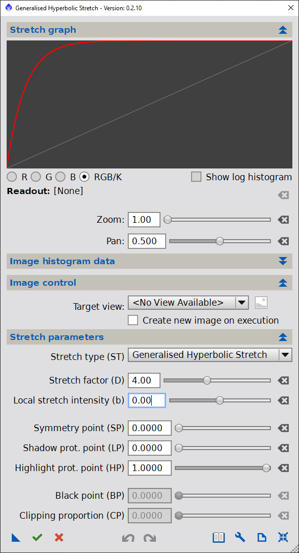
Technically, move b to the left of 0 utilizes the integral form of the generalised hyperbolic equation. The special version, for b=0, of the integral equation is identical to the base form - that is an exponential stretch. As b reduces to b=-1, the form of the stretch becomes logarithmic, rather than exponential. Note that this is the fundamental form of the popular arcsinh stretch. While similar in form, the arcsinh stretch employs a modified form of a logarithmic stretch, which is almost identical to a stretch performed using b=-1.4. For b<-1, the stretch becomes increasingly gentle and the contrast redistribution is less dramatic. For b values less than, say -3, the stretch function because almost independent of the vaue of D employed and extremely gentle, adding only a subtle amount of contrast at SP and otherwise almost "linear".
These subtler, gentler forms of the GHS are ideally suited to final stretch adjustments made to the image and in general, a progression of stretches performed using the GHS should be from higher positive values of b to lower, more negative values of b towards completion. The key to performing this successfully is to keep an eye on the histogram, with a periodic query of the preview of pre and post stretched images to ensure that the stretch is accomplishing what you want. In fact watching the histogram when learning the script is the best way to familiarize yourself with all of the controls.
It may appear, at first, that negative values of b (<=-1) are the kindest on stars and bright portions of the histogram. This is true, but not if multiple repeated stretches or large stretches are envisioned. For example, if you were to use a large D to accomplish a stretch of a linear image, you might find that the repeated stretching with large D factors, such as what may be required when starting with a linear image, that in the end - a better initial stretch would be to use a single stretch with b>>1.
3.2 Highlight Protection (HP) and Lowlight or Shadow Protection (LP)
The highlight protection (HP) slider's main purpose is to provide protection to highlights (brighter areas or stars) by making the stretch linear above the value of HP. It does this by stopping the decline in slope to the right that is inherent in the GHS transforms and keeping that slope constant (linear stretch) to the x,y=(1,1) point. The slope that is adopted is the same slope that is generated by the GHS transform at the HP point, in order to preserve slope continuity and avoid stretching artifacts. In terms of the highlights themselves, they will continue to be stretched, as they must be brightening more than the pixels below the HP point, but at a reduced level than would have been without HP protection. This highlight protection is over and above the normal highlight protection offered by the GHS alone in your selection of b, and can be used to great effect, even when using a (b=0) exponential form of the transform. However, this highlight protection is a compromise, and even with its use mulitple stretches can cuase star bloat, and a loss of their gaussian look may still occur.
Figure 11 — Introduction to Highlight Protection Slider, (HP)
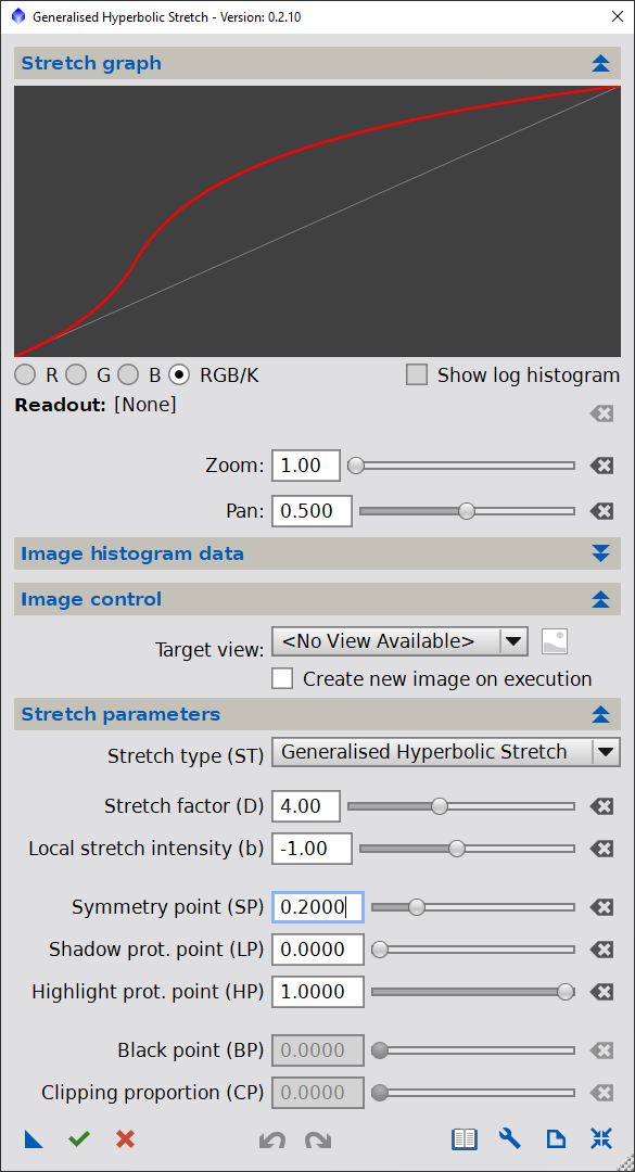
- Exponential, D=4, b=-1, SP=0.2, No highlight Protection, HP=1
- SP=0.2, HP=0.8
- SP=0.2, HP=0.6
- SP=0.2, HP=0.4
- SP=0.2, HP=0.25
- HP=SP=0.2 - Partial Blackpoint Adjust with transition
- Alternative to Black Point Adjust
- BP Adjust with transition to stretch
- BP Adjust with harsh transition
- BP Adjust with gentle transition
Mousing over the first five images in Figure 11, it is apparent that when HP is lowered, not only does the span of protection increase, but also the degree of protection (in terms of slope or contrast). As HP is lowered, the amount of stretch being applied above the HP point is reduced. The effect is subtle at first, graduating to a greater slope covering a larger span..
At a certain point, (at approximately HP=0.25 for these parameters, the stretch virtually becomes the identity (y=x) and very little stretch is applied above HP and the pixels values are unchanged above the HP. At this point, the stretch becomes a compression (dimming) of just those pixels below HP.
By continuing to move contrast from the left side of HP, to the right hand side and the stretch transform will lie below the y=x when the point where HP reaches SP (symmetry) point, - maximum protection to the contrast on the RHS of the histogram.
Backing up to HP=0.4 by mousing over this image in Figure 11, while examining the LHS of HP shows that the stretch occuring here is reduced as HP is lowered and vice versa. Using the identity line as a reference, one can see that parts of the stretch transform dropping below the y=x line when HP=0.4 in this case. Note that these pixels are being dimmed, rather than brightened. This illustrates the second role that HP plays in the stretch transform design - which is to push down or raise the stretch transform on the LHS of HP.
As the RHS of HP approaches the identity line, the entirety of the stretch of the LHS will lie below the identity line resulting in a dimming of this part of the image, although to various degrees. Reaching the point where HP=SP, the RHS has "stolen" all of the contrast from the LHS that it can and the LHS essentially lies very low indeed (close to 0). Unlike the linear-prestrech equation the information in this background data is not lost entirely clipped and can provide for some trasition from blackness to background. In Figure 11, for example this is seen in the sixth image down. Some adjustment to b and D can make the points lie even closer to the floor and this, in effect, will perform a "Linear Pre-stretch" equivalent on the data and forms the second method for shifting the entire histogram to the left, while linearly normalizing the histogram on the RHS, as illustrated in the seventh image in Figure 11. (Note that many of the curves illustrated in Figure 11 represent large stretches for illustrative purposes. It is more likely that you will use signficantly lower D values in practice).
The recipe to perform this black-point adjust is to first set SP to the desired black-point position, and then set HP equal to SP with a setting of b=0 or above, a reasonably high D value and executing.
As we have seen, however, that by moving HP a small amount to the right of SP, one can effect a desired transition from background to foreground, as illustrated (in an exaggerated way) the methodology to do so. If you want a "fade" from foreground to background, use a negative b and small D with HP backed off of SP to the right . If you want to see the foreground "lift off" of the background, then a higher b and larger D should be used. SP and HP should just span the background level noting that the distance between SP and HP will also control the effect.
Having established the effect of the HP slider, the role of the Lowlight (Shadow) Protection Slider (LP) should be apparent. LP reserves contrast from the GHS portion of the transform and applies this contrast to the lower portions in the form of a linear stretch, using a slope consistent with the start fo the GHS transform portion of the stretch. In this way LP does essentially the opposity of HP. LP retains the some of the contrast in the shadows, rather than potentially darkening them to the point of losing this detail. Of course, LP cannot be raised above the current level of SP, nor SP reduced below LP.
Mousing over the first 5 images of Figure 12 illustrates the role of LP. In these figures SP has been set to 1.0 so that the entire transform is in inverse stretch (compression?) mode.
Figure 12 — Introduction to Lowlight / Shadow Protection Slider, (LP)
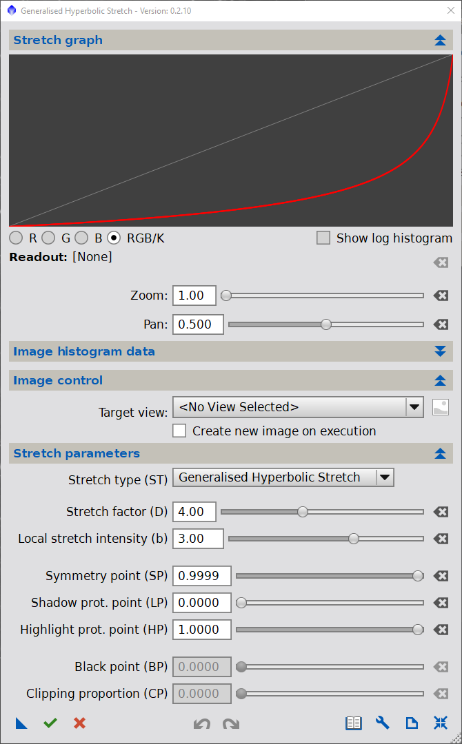
- (Familiar) SuperHyperbolic Inverse, D=4, b=3, SP=1, LP=0
- LP=0.5
- LP=0.75
- Bright Star Rescuer, D=4, b=3, SP=1, LP=0.875
- Identity Transform, LP=SP=1 (or HP=SP=0)
- Contrast Insertion - Hard on Stars & Background
- Contrast Insertion - Better
- Gentle Contrast Insertion - Best
- Harsh Contrast Insertion - Problems?
- Bilinear Stretch
Combining the use of SP, LP, and HP, we can see that any general application of the GHS script can be subdivided into four regions. Below LP, the stretch is linear (constant slope). Between LP and SP, the slope (contrast increases) to a maximum governed by the D and b at SP. Above (to the right of) SP, the slope declines again and until the point HP, where is left constant again and above HP, the stretch is again linear. I suggest playing with the sliders and at the same time, watch a histogram of a (prestretched image) loaded into the script itself. In this way, the effect of all five inputs into the GHS stretch equations can be viewed. Additionally, to reduce the number of parameters, you can do the same using the HT equation or the arsinh stretch equations (both assume a constant b value in their formulae), to see what the functionality of LP, SP, and HP bring to these equations too, via this script.
The use of these three point, working in tandem, can create many special functions to achieve specific results with your image. Since the placement of SP, LP, and HP control the overall brightness added to a stretch, they can be used is a series of stretches where overall brightness is added to an image followed by brightness taken away from the image by changing the input. In this way, contrast can be added to specific points in the image, near the completion of the stretch sequence, without changing the overall brightness of the im
The importance of this stretch-unstretch recipe will be revealed later, as will some of the ways to manipulate the five GHS controlling parameters to achieve specific results. However, to avoid making this primer's contents too dry, here is a recipe you can use to rescue bright stars that may be losing their Gaussian shape and being replaced by bloated circles. The earlier in the stretching progression you can recognize star bloat occuring, the more successful the star rescue will be. The function also depends upon stars not being severly clipped:
- 1) Choose a D and b of mid to mild strength
- 2) Move SP all of the way right to 1.0 - this will add the most contrast within the stars - exaggerating the remaining contrast in the stars
- 3) Move LP slider to a point just below where, on the histogram, the pile up on the right side of the histogram indicates that the stars are bloating. A log view of this histogram is best. A value of 0.9 might be a first guess. LP here will confine the non-linear portion of the "antistretch" to the problematic stars, while minimizing the effect on the remainder of the image, below LP; conduct this stretch - you will see the stars restored
- 4) Conduct a gentle stretch, with b below 0, a very modest D; SP and LP at zero, and a HP, now set at the level LP was set at (0.9?). This will recover the image brightness lost in step 3)
Conceptually, what is being done here is an asymmetric stretch of the data. When SP is at 1.0, the image is being dimmed with the majority of the contrast being placed in the brightest stars. In step 4, a much more gentle stretch is used to "rebrighten the image" but redistributing the contrast in a more gentle manner, so as stop the stars from returning to their over-stretched state.
3.3 Reversing the Stretch and the Inverted GHS transforms
At this point, it is worth mentioning that the a sixth, special form of the GHS equations has been included in the script that mathematically reverses any GHS transform previously applied to an image - ie. moves backwards through your stretches.
The easiest way to utilize this script is to perform your stretches as recorded in your logs (indicated by ST=0 with the parameters listed) in reverse order (this time with the inverted GHS transforms selected) to get to the point where you want to change the forward stretch sequence and move from that point into a different direction. Note you can also do this, of course, with the undo facility both within and outside of the script itself - but not if you have exited Pixinsight without saving your intermediate points. This is why you should maintain your log file. Figure 13 illustrate the forwards stretching using the GHS formulation, followed by the inverted stretch to get back to the starting point. Note that the inverted stretch is a mirror image about they y=x line.
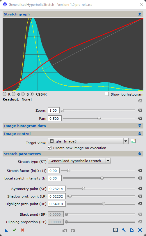
Of course, you could just use the Inverted GHS transform on the image in a non "back up" manner, just to achieve a special effect. However, you will note that all of the roles of the main parameters are reversed. Using the inverted formulation, SP selects the point where the contrast will diminish the most while D and b have the opposity effect as in the forward, normal transforms. Also, the selection of SP, LP, and BP can be more difficult as they refer backwards to the stretch you are about to undo which, at this point, is a moving target. I, myself, have very limited experience in performing inverted GHS stretches on images because usually they don't look good as they are, by nature, designed to undo our stretching work. Feel free to try.
Where they can be useful, is performing an asymmetric stretch, that is conducting a stretch with a set of parameters and then undoing it by changing one or two parameters so that the "undo" is not identical to the "do". This has the potential of manipulating the image in a way that leaves the effects in the original operation intact, but removes any unwanted side-effects that resulted. Again, I see the potential but haven't fully explored this myself. Feel free to try.
As an aside and for those who may be using their cameras to do photometrics or measuring the absolute brightness of objects, camera linearity is of great importance. I see this facility as having potential to correct cameras from any systemic non-linearity. Using a benchmark linear image together with a camera view of the image, it may be possible to describe the non-linearity of a camera by comparing the histograms of the linear image itself with somewhat non-linear camera view. If the difference can be described by a GHS transform, then the inverse function can be used to correct for this camera's non-linearity to make photometric evaluations/observations using the inverse transform, provided that the non-linearity is systemic to the camera.
One note about this feature, it is less precise that using the "undo" button - either within the script or in the main workspace. These "undo"s are accomplished by recalling temporarily saved images that were put into memory prior to execution the stretch in the first place. When using the inverted GHS facility, an actual transform is applied. This means that the inverted GHS facility is subject to numerical precision issues such that the result, while analytically an "exact" undo, digital numerical issues may add some noise, especially when repeated several time, or restoring dark background brightness or over-stretched stars.
3.4 What could possibly go wrong?
Based on the nature of the equations and the four properties discussed in the initroduction, it is difficult to mess up a stretch sequence but it is definitely possible. Before encountering a problem it pays to make sure that it will always be a small problem. The first way this can be done is to start any new process of data transformation (with either the GHS Script or any other process) using a clone. I generally create a new clone whenever undertaking a new process, changing and appending the name of file first with the last process conducted on it and iconifying it once the clone is created. Saving some of the intermediate results as major junctions in the workflow is also recommended.
Within the GHS script, there are many additional ways to ensure you don't spoil your data by taking a wrong turn. Firstly, you are given the option to create a new image or overwrite the existing image. In doing the former, you can always revert to the previous image if a mistake is made or using the undo command if the latter. Next, is to make use of both the histogram and the preview image to find out where you are and where you are going. Check the preview often. Query the image preview, and match the pixel values to where they are on the histogram. You can then use the histogram preview to see where that point will lie in the transformed image. Then look at the preview once again to see what the proposed stretch will do to it.
When exiting the GHS script, you will be prompted to potentially save a log file. I recommend saving this file - it is a simple ASCII text file that contains a detailed account of GHS script stretching including the names of the target files, resultant files and all of the parameters necessary to reconduct the stretch. This log file can be used in many different ways, and actually brings science to the stretching process. Steps can be repeated to a certainly point, or taken past a certain point start either with the original linear image. Sometimes, it pays to move forward with a different stretch (such as contrast insertion to the stars described above). I have found that if a stretch conducted does what I intended, but its execution also had unintended consequences, there is likely a follow-up stretch that can be undertaken to reverse just the unintended ones. This is the "asymmetric stretching" methodology.
The best final histograms, in my opinion, are those that start at zero, rise to a single dominant peak around 0.2 to 0.25. The histogram should then decline more modestly, with possible undulations and minor peaks and valleys towards x=1, with a possible minor peak at the RHS representing clipped or overstretched dominant bright stars. You should have this shape in mind when undertaking the stretch sequences while keeping one eye always on the histogram to make sure it is going to the right place.
A large gap on the left side of the histogram is likely a result of too much contrast being placed between 0 and the start of the pixel value data. You can fix this by doing one of the forms of black-point adjustment. This gap, in most cases represents a "waste" of dynamic range or contrast that likely is better spent in the guts of the image. In a few cases, it may be there because you don't want the background to be dark. I suggest getting rid of the gap as soon as possible. Often I try and remove it even before the first stretch to non-linear - by selecting an ultra-low clipping point (0.0001 or the minimum pixel value). If not practical though, I definitely remove or reduce it after the initial large stretch.
We have discussed star bloat and its indications already. If your initial histogram (of linear data) shows some star clipping, be sure to use HP protection. A large b value on the original stretch will also help keep the overall stretch large, yet reduce the amount of stretching applied on the RHS. Finally, an application of the star rescuer stretch will help enourmously, followed by a gentle stretch to restore image brightness.
Another issue that may appear is that of noise. When stretching the signal, you are also stretching the underlying noise - making it much more visible. Due to numerical precision reasons, you may be also adding numerical precision noise, (called numerical dispersion). Always keep an eye on the image (using STF), checking for noise. There is nothing wrong with pausing, mid stretch sequence, and exiting the script to perfrom a noise reduction process, and then resuming the GHS script. Bear in mind, however, that the process of noise reduction also can remove some signal.
Perhaps the most incideous form of problem that can occur with the GHS script is that of pixel "bunching". This will manifest as a lack of contrast between pixels within the image and will appear as a haze over the image, or leaving the image looking very flat. To some degree, pixel bunching will occur because it is caused whenever the stretch function has a curve to it which is pretty much always. Whenever a stretch curve is concave down, or to the right - pixels will be pushed rapidly around the bend (where contrast placement is greatest), but then the stretch will diminish as the transform flattens, and pixel values will move less, causing pixel values to "catch up" and bunch up somewhat to the right of the curvature. The opposite will occur when the transform is concave up and to the left, However, in this case the bunch up will occur to the left of the curvature.
The GHS transforms will generally avoid severe bunching that can occur with the non-judicious use of the Curves Transform, but nonetheless can occureven though the GHS transform slopes will always be greater than zero even when severe curvatures are applied. As a general rule, try to avoid severe curvature stretches in the mid-range of the histogram.
The gathering of pixels can form an apparent peak in the histogram. A small one might be Ok, or if it happens once you might be alright by adding some contrast at this peak. However, this may cause a different peak to appear elsewhere and you should avoid playing Whack-a-Mole on histogram peaks or image "flat areas". It may be better to back up a stretch or too, and trying to use a smaller b as excessive curvature often arises from use of too high a b factor, when the problem could be avoided by using a higher D or other adjustments to SP, HP, or LP. As a rule, I tend to use ever decreasing b factors through my stretching program, and only breaking the rule for application of one of the "special transforms" previously discussed. Overall, watch for excessive curvature in the transforms (other than the initial transform where it often pays to use a higher b).
It is useful to remember that no amount of GHS stretching can accomplish what local stretching or local dynamic range expansion can perform. I am thinking of HDRMultiscaleTransform (HDRMT), Local Histogram Equalization (LHE), GradientHDRCompression (GHDRC), or even Dark Structure Enhance (DSE) script here. These local transforms do alter pixel values, but not just based on their starting pixel values alone. They also look to the pixels surrounding it to provide dynamic range in the middle of the structures. The GHS stretch cannot accomplish what these processes can, so don't attempt to try.
My limited experience with the GHS script has also shown that the best overall stretches are achieved with few steps. It is the nature of the hyperbolic equation that many executions, employing a variety of input parameters, trends toward the equivalent of a single application of exponential stretch. The law of diminishing returns is in play - while you are free to refine your stretch as much as you want - starting from linear and moving towards a full stretch employing a multitude of small, gentle stretches may not be the best strategy.
I have had a much better results by employing one or two large initial stretches (with a large D b and an appropriate SP) that gets most of the way to the final brightness. Be bold in this first stretch it will likely be best at maintaining colour saturation and covering the histogram with the data you want to show. I target a peak histogram value of 0.2 ish and look at the results. You may want to adjust parameters somewhat and try again. I then employ of the forms of blackpoint adjustment and potentially another step to adjust the background transition. A couple of further adjustment are done to highlight the parts of the image that I want using low b factors and judicious placement of SP, HP, and LP will take the histogram peak to 0.25. Once close to my desired peak levels, I may employ one or two asymmetric stretches to fix brightness levels in the rest of the image, potentially including a star rescuer, and I will be done. Again as a rule, I will try and do all my stretching in 7 steps, never more that 10, but even fewer if possible. If I reach 10, unless the result is magnificent, I will start again - reviewing my log file to make sure I learn from my mistake(s).
3.5 Incorporating the GHS into your Workflow
Of course, achieving this will depend on what your current workflow looks like now, and what equipment, filters and camera you used. I will try and keep this overview highlevel, focusing on where the GHS script can be used in addition to, or instead of your existing stretching functions.
Fundamentally, my process consists of
1) Creation of two primary images: a monochrome image that contains the best of my luminance data and a colour image which contains the colour information that I want to use.
To start, this will involve combining and calibrating all channels, whether they are RGB, Narrow-band false colour, or luminance (or combination therof. For monochrome cameras, I may extract luminance channels either from RGB or narrow-band data to combine with my stand-alone luminance images to create a "super-luminance file" (SLUM) file. For one shot colour cameras (OSC), I may simply extract a luminance channel that will act as my luminance. The point of this exercise is to create two images for further processing towards the final result: a luminance image and a colour image that can be processed in separate workflows and combined towards the end to create my final image.
The reason for this separation of colour information and monochrome is that the workflows conducted on each are likely very different. Some processes focus on luminance (such as deconvolution and local dynamic range enhancement) are difficult to control on colour images. Therefore, it makes sense to "divide" and conquer and execute these processes on the luminance channel alone. For the colour image we can focus on colour, ensuring that the final image has the best of both worlds.
Before proceeding further with either the colour or lum images, it is best to perform noise reduction on them, as stretching will enhance both noise and signal. For this process, I may wish to employ a luminance mask.
To create this mask, I load the luminance file that I am proceeding with into the GHS script and proceed with the process outlines in the walkthrough section of this primer. My target for the histogram peak is 0.25 . Usually I can get there with one stretch. I may adjust SP slightly, but generally leave b=0, as this adds protection to the brightest stars by the mask to an image. Upon execution a new file will be created, that I rename my luminance mask, it will be no-longer be in "linear form". Before proceeding to use this mask as a noise reduction mask, however, I may perform my favourite noise reduction routine fairly aggressively because using a noisy mask can create additional noise.
Once this mask is created, I can apply it (in inverse form) to execute linear noise reduction on the colour linear image(s).
2) Perform linear processing on the luminance image. In particular, deconvolution requires that the image be linear, so it must be done before GHS makes the data non-linear.
While the GHS is not involved at this stage, it plays a major role in mask creation.
The second mask that is generally needed is an object mask. To create this mask, I load the previously created luminance file into the GHS script. The SP parameter is usually set around the 0.2 level, I then use D and b to shift pixels values to the far right and left. I may even employ the LP and HP sliders to leave some gradation in the image. Alternatively, I can essentially binarize the mask by employing a very large b and D to the stretch while leaving LP and HP at 0 and 1. This all depends on the mask that I want.
Starmasks can be created using either the "Star Mask" or "StarNet" processes in Pixinsight on the previously created luminance mask. As a general rule, I try not to binarize using the Star Mask process preferring the control over where the binarization cutoff take place and how strongly it is binarized with the GHS script. Binarization of a StarNet star mask is also easily done with the GHS script.
The Star Mask process sometimes does not capture the largest, brightest stars in my image. If I am using this process to create a "deringing mask" for deconvolution, I may augment the stars it finds by using a combination of: the GHS script to isolate the brightest stars, the range mask process to remove residual brightness from the image, and finally Pixelmath to add these large stars back into the Star Mask process range of stars.
I may also apply a modified version of my object mask to my linear luminance when conducting deconvolution. This can be achieved by using Pixelmath to subtract my "custom" star mask from previously created Object Mask. This mask is not just good for deconvolution, but is also handy down the road for executing non-linear process post stretching.
Once this is done, I have all the masks needed for deconvolution and I proceed to execute this process. Finally, I apply my luminance mask to execute noise reduction on the deconvolved luminance channel prior to stretching.
3) Stretch the Luminance Channel
Both luminance and colour images need to be stretched to get to the final result. What I like to do is use the histogram of the stretch of one as the target for the stretch of the other, as this will produce the most natural overall recombination of LRGB in the end. Generally, I start with the luminance image stretch first. This is because deconvolution may have changed star brightness causing it to require additional star protection compared to the colour image. Secondly, there will be other non-linear processes that will be applied to the luminance channel that may alter this "target" histogram.
We should now be familiar with conducting the stretch itself - it is the main focus of this primer. I always try to keep my eyes on the histogram and check the images for noise.
Before proceeding, however, it is worth mentioning the ability to use masks with the GHS. Although the functionality to apply masks to the target image does not (yet) exist within the script itself, it is perfectly fine applying a stretch to a masked image. Because the GHS exists within a script, it is not a process, so the mask must be applied when outside the script.
Application of the mask to the stretch is governed by the same rules as used in the Pixelmath process, ie. if the GHS script is instructed to create a new image, the applied mask will be ignored. However, if this box is left unticked and the GHS script is asked to overwrite the image then the mask will be applied to the stretch. Before using a mask on a stretch, you should ensure that the mask has been aggressively denoised, and subtle masks with sufficient smoothing work best.
I have successfully used both luminance and "colour" masks generated with the ColorMask script successfully with the GHS script. However, as a general rule, they should not be needed to enhance features using GHS.
A colour mask can be extremely helpful when features appear in the colour image only, when they are not apparent or very faint in luminance alone. A subtle stretch with a colour mask, can provide that bit of contrast from the background that can make the feature pop in the final image. Generating such a mask may require a quick stretch of the colour image first, just to extract the appropriate mask. However, as a general rule, they should not be needed to enhance features using GHS.
Note that the mask will continue to be linked to this now-stretched image. To create a unmasked version, you can simply then create a new image by ticking the box and using an identity stretch. Also note that the "undo" recipe to work on the stretched image, an inverted version of the mask must be first applied to the stretched version.
4) Conduct Non-Linear, Local Processes on Luminance Image
The non-linear processes here represent HDRMT, LHE, Sharpening, Noise Reduction and others and can be performed on the now non-linear luminance image. The masks created previously are excellent for this additional work. It is likely appropriate to conduct apply noise reduction and sharpening to the luminance channel before combining with the colour image.
After these process have been conducted, a minor stretch getting to the overall brightness desired may be necessary. Note that another minor adjustment will likely be desired after combination with the colour image.
As of writing this script, I have not yet conducted tests to see the effects of "overstretching" an image using GHS, prior to conducting non-linear local processes on it, followed by an inverted GHS to restore the image can help with the local processes. I feel though, that this has the potential to add value to an image (and is essentially the form of an "asymmetric" stretch.
Once these non-linear processes have been conducted, I re-examine the histogram, taking mental note of the salient features of the histogram, as this will form the target for the colour stretch.
5) Stretch the Colour Image to roughly match the overall intensity of the Lum image, Stretch/Adjust Saturation, Adjust Hue
In terms of the stretch itself, we should apply all of the principles previously discussed in this primer, with a target of matching the brightness profile, or histogram of the previously stretched luminance image. It is not important to get this exact, and in fact it will likely be impossible because the colour image did not go through deconvolution, nor any of the other local histogram adjustments. Once you are close, a final linear adjustment of the total colour brightness (by extracting the "final" luminance, performing a LinearFit process to match the stretched luminance image, and then channel combination to recombine with the saturation and hue channels) can often get you close enough.
Just getting close enough, in some ways, makes the stretch of the colour image easier than the luminance. In theory, you should perform roughly the same stretching parameters that were recorded in you log file(s), but this usually is only a guide and at some key points you may find you have to depart significantly from the luminance stretch. Overall, the same kind of stretch transforms should be performed - ie a large, high b stretch at the beginning, followed by lower, more negative stretches afterwards to get to the same profile. As with the luminance image, you should also check the colour image for both noise - but this time "colour noise" as well as "luminance" noise. You may find it helpful to perform noise reduction mid-stretch but almost definitely after the stretch sequence.
What makes the stretch of the colour image more difficult, in some ways, is that you need to keep an eye on the colour saturation. It is the colour image that will provide the colour information to the final image. There are multiple ways that colour information is represented in an image, the most common way is through separate red, green, and blue channels - corresponding roughly to the cones in your eyes that see colour. (Note that images get away with this, because your eyes/brain cannont distiguish between, say "yellow" light and mixture of "red" and "green" light since they both elicit the same proportional response in your the red and green receptors and you don't have a "yellow" receptor). These proportions of these red, green and blue are represented in the image data in these separate red, green and blue channels.
It is on this RGB colour information basis, that the GHS script is set up. When a stretch is performed using the GHS script in default K/RGB mode, the same stretch is performed separately on each of the colour channels, and the net effect is to proportionally stretch each of these channel so that the colour remains the same regardless of the colour information. For many images, after colour calibration, there may be no need to make any colour adjustment as the stretch is performed since the proportionality of the separate channels is maintained with the stretch. In these cases, you only need focus your colour stretch (and noise) when stretching the image.
Another popular way to represent a colour image is the "LSH" model. As with RGB this takes used three channels to represent the image. The first one, luminance, is used to represent how bright each pixel is. Suffice to say, this channel is an average of the R, G, and B channels in the RGB representation. The second, saturation channel, roughly equates to the proportional difference between the R, G, and B channels (or standard deviation of the R,G,B that represents the colour intensity. It the variation or standard deviation of the colours is low, then the pixel will appear "whiter" or "greyer" or "less vivid" than if the standard deviation is high, where there is a large difference between the individual colour contributions resulting in a more colour intense, or colour saturated pixel. The third and final channel, Hue contains the information about what colour is being displayed which basically determines which of R,G or B is most and which is least intense. Overall the LSH model contains the same information as the RGB model, only in a different format. With Channel Combination (CC) process and Channel Extraction (CE) single channels from both models can be extracted from or recombined to produce the image.
During the colour image stretch, after stretching the overall luminance to match the luminance image, it is this saturation colour that we are most concerned about. There are several reasons why you may want to change the colour saturation in your colour image during or after the stretching purpose, but for many cases this may be unnecessary. Firstly, the information from your filters and/or camera may not contain enough saturation to your liking - these pieces of equipment are not perfect. Secondly, as we brighten an image, we do not percieve colour the same as some of our receptors might start to get "saturated". Thirdly, when we ultimately combine our image with our luminance channel, our saturation will be diminished somewhat, although there are controls in the LRGB Combination process to adjust for this. Finally, the colour saturation is a also a matter of taste. Any saturation adjustment to images are best made during the stretching phase, as just with luminance, saturation adjustments on linear images is very delicate due to the tight histograms.
The Hue channel is generally set by the pallette you want to use (assignment of filters to R,G, and B channel) and/or colour calibration performed in linear mode. There are many tools available to adjust hue independently of the other channels in Pixinsight. The best place to make dramatic hue changes in linear mode, prior to colour stretching, and once again, Pixinsight has several tools to make such changes. However, during the stretching process may reveal undesireable "hues" by brightening the underlying luminance. As with saturation, subtle hue corrections should be made as they are revealed and the histogram becomes less tight.
The GHS stretch does not currently (next release?) have the ability to work on the "LSH" channels independently. Rather, it operates on the RGB mode. This can be use to great effect in correcting for any Hue issues that might arise during stretch - which can occur most often during the stretch of narrowband images or images that were (deliberately?) not colour calibrated. Such adjustments are best made using the histogram (to allign or deliberately misallign) the individual R,G, and B channels. To invoke this hue correction, one can select which channel, (R,G or B) to apply a stretch to. In general, unless you belong to the impressionist school, you will likely want to make gentle corrections using a large negative b and small D to finally adjust R, G, or B. This is a fantastic way to get rid of unwanted underlying colours that may crop up during the stretch.
More frequently, you may want to just adjust the saturation channel. However, when adjusting for R,G, or B with the GHS script in its current version will adjust the luminance, saturation, and hue all at the same time. This may not be what is desired. What may be needed is an independent asjustment to the saturation itself. GHS can do this, but it takes a few steps. first the script needs to be exited, the saturation channel extracted using CE, the GHS applied to stretch the saturation channel as a monochrome image, the RGB image put back together using CC, then reload the image back into the script. The GHS script will indeed perform a precise stretch in this manner, but currently will not perform this in an "automatic" sense.
It is more likely that you would perform such "saturation" stretching using the Curves Transform (CT) process in Pixinsight. With the CT process, the extraction of the saturation channel is done automatically, allows for the preview of the saturation stretched image, and puts the RGB file back together automatically once the stretch is performed. This is the method I now use, performing a saturation stretch (increasing the standard deviation of the R,G,B channels) after I have matched the colour to my luminance image using GHS. I may also perform a saturation stretch at an intermediate stretch, if needed. A final, saturation strech is often executed after the luminance and colour images are combined.
The author of the script and myself are still considering the best way to do saturation stretching in the GHS to make it a "one stop" stretching script, but there are a few alternative to doing this. Consequently, we have put this component aside for the time being.
Arcsinh Stretch (AS) Process - A Digression
The Arcsinh Stretch is a popular stretching process currently available in Pixinsight to stretch both the luminance and saturation channels at the same time. Although the title of this process suggest that this is something that the nature of an arcsinh transform is responsible for, it is not completely true. Indeed the arcsinh stretch is a gentle stretch on its own, (large negative b equivalent), that is gentle on stars for very small stretches. I, myself, would generally start a stretch with a large Arcsinh stretch because I liked what it did to increase colour saturation.
The AS process achieves a saturation stretch by first applying the stretch to the luminance channel (and not the saturation channel, as you might think). Then the actual stretch factor is determine by dividing this stretched luminance by the original luminance - essentially determining y/x for each stretch. Then this stretch factor is multiplied by each individual RGB colour channel. The result is for every pixel, the colour channel that has a slightly highest value will be stretched more, and the channel with the least intensity will be stretched less, resulting in an overall increase in the standard deviation, or colour saturation of the pixels. The AS process effectively stretches both the brightness and saturation at the same time.
The same process can be theoretically be achieved with any stretch function, included any of the GHS stretches by first stretching the luminance channel, and then applying the same stretch factor normalization and multiplying the individual channels by this stretch factor. This second step, must currently be done in Pixinsight by doing it via Pixelmath as shown in Figure 14. Note a small value has been added to the unstretched luminance image to avoid any divide by zero error. The value can be increased further to avoid too much stretch to very dim pixels - similar to determining the "black point" in the AS process itself. Once the Pixelmath has been applied, the image will be stretched in both luminance and saturation. Note that a very gentle stretch of the luminance should be applied (such as the arcsinh stretch itself) to avoid artifacts, particularly in the stars.
At one point, I liked what the arcsinh stretch was doing to my colour image saturations so much that I always used it. More recently, I have switched back to saturation stretches using the CT process. The reason is that the AS, in my opinion, is trying to do too much at the same time. The actual arcsinh equation (the equivelent of b=-1.4 in the GHS equation), is a very gentle stretch, particularly at the extremes of low x or when x>0.5. In addition, the contrast redistribution is very low when using a b<-1. If a more positive b is used, the stretch at low values will create colour artifacts in this method, and if the mid to high values of range is stretched too much, artificats in the brightest pixels will appear because the standard deviation will be stretched too much. The AS stretch forms a good stretch that will avoid these artifacts even when performed with a reasonably high equivalent D or performed repeatedly. Unfortunately this is the opposite kind of stretch we want to initially perform on luminance to get the best results. Repeatedly performing such an arcsinh stretch / negative b factors, or with large D's will result in a very poor luminance stretch, potentially over-stretching stars.
Instead of using the AS stretch on the linear image, I have found that I can get more than ample, and just as good saturation results with the CT process, after using a large positive b on the initial stretches to get luminance correct. If I still want to use the AS methodology, there are a few alternatives to consider
- 1) Use the AS process after the initial stretches. The effect of the AS process will be diminished, but still effective. You can even overstretch the luminance at this point, and then undo the arcsinh stretch by employing the invert - unstretch - invert recipe to the image, applying SP=1 to the equation to return the overall brightness to the correct position.
- 2) Use the PixelMath equation, calculated at the linear stage. Once the Pixelmath process is applied, one can also undo the stretch on the colour image using the GHS equation. Furthermore, by using the arcsinh stretch or negative b equivent, one can control where the saturation stretch occurs with the additional LP, SP, and HP sliders.
- 3) Use the GHS script to stretch the luminance directly, followed by the Pixelmath method to add saturation. By using the inverted GHS functionality, the gentle stretch can be be removed from the image, leaving the saturation enhancement behind Then, a more practical GHS stretch can be conducted to better serve the luminance or image brightness objectives. Note I have used this method a few times and it has been successful.
I have tried all of these, but now find stretching the saturation the most convenient. That leaves me with the freedom to choose the GHS parameters I like best to achieve my desired luminosity results on the colour stretch.
The options and processes discussed here are all being considered for the next version of the GHS script.
6) Combination of luminance and colour images
This utilizes the stretched and processes luminance and colour images to combine into one (fantastic, I am sure) image. This is best done using the LRGB combination process.
7) Tidying Up
This amounts to any additional processes you wish to perform on the combined image. For me, this generally consists of at least, a one last crack at stretch adjustment using GHS looking at stars, background and any features I want to hide or standout. A CT adjustment of colour may also be desired.
I now also ensure that my GHS logs are named appropriately so that I can save how I stretched the images in case I want to rework them at a future date.
Please feel free to post whether you used the GHS script and how you found it. That way the authors can take some gratification in helping with your success and enable us to improve it in the future.
4 Generalised Hyperbolic Equations used in this script
[hide]
If you are interested in the form of the GHS equations, how the forms relate to one another, and how they relate to the stretches performed by the HT and Arcsinh process, then review Figure 15, mousing over first the parameter definitions, and then the specific forms of the various equations. The form depends on the b parameter entered for the GHS, while the HT and arcsinh have an equivalent "b" parameter built into their formulation.
Simultaneously, these equations provide a lot of flexibility in performing non-linear transformations in a natural way and are self-limiting, in that regardless of the form or inputs use, they have properties conducive to the stretching process and artifact avoidance.Specifically, one can employ the stretching routine knowing that the transformations:
- are true functions (not relations): the mapping of stretched results is 1:1 with the input image: this allows for the ultimate reversibility of the transform. A GHS stretch can be reversed by selecting the "Inverse GHS" selection (the 6th stretch type (ST=5)) in the stretch type selection pull-down.
- all yield a stretched result of 0 for input of 0 and a stretched result of 1 for an input of 1: there is no clipping of input data and, within the limits of digital resolution, no loss of data from the original linear image.
- are increasing between 0 and 1 - positive slope:. This preserves the rank order of all the pixels in the image. This may be important for the scientific application of images where relative brightness may be important.
- are all step-wise continuous and also have stepwise continuous positive first derivatives (slopes): This avoids flat spots in the transformations (reducing the bunching up of the histogram and "flat" looking results, sudden artificial looking spikes in the histogram, or inverted looking image parts.
- are analytically integratable/differentiable, allowing for stretching functions that are limited only by numerical (digital) precision and not reliant on "spline fits" or approximiations that can also yield artifacts
Now, there are occasionally times where one is fine with intentionally violating these constraints and certainly these equations provide less flexibility than the Curves Tranformation (CT) tool, which essentially allows for complete freedom. Just be aware that use of the CT tool can result in unwelcome artifacts, lack of a reversible and reproducable mathematical trail from input to output. Other than these constraints that are designed to provide a "safe" stretching environment, I hope you will see that the flexibility to perform various transformations is almost limitless.
The first image just contains the parameter definition as described in the earlier sections of this document. One important fact to note, is that the "D'" stretch factor is not identical to the "D" as described in the equations. D' is in essence the logarithm of D applied in the equations. This mapping of D is to allow for large D to be readily entered with the slider for large stretches, and fine adjustment of D needed for small stretches.
The second image is the form of the exponential stretch, or the limit of the GHS when b approaches 0. A b=0 is the dividing point between the base form of the GHS and the integral form. This is because the integral form of the exponential stretch is the same as the base form. This form describe the increase in product / decrease in reactant of a nuclear decay or a batch chemical reagent/product concentration, the growth rate of an epidemic, or even the present value of money in a continuous compounding rate bank account, or subject to inflation. In stretching, its magic is in the fact that it is self-similar at all scales. In practice it is only used for gentle image stretches as it can be unkind to stars in a forward stretch, or the background in an inverse stretch. The contrast applied at x=SP is proportional to D.
You will note that for each of the images describing each equation form, the actual equation have been normalized to run through the points at (x=0,y=0) and (x=1,y=1) - suitable for non-clipping of data. Thus the level of stretch at any given point x,y is dependent on the full set of equation parameters. Each of the equations used is analytical, and has an analytical first derivative and that derivative is continuous throughout the applicable range. These properties maintain the data integrity and repeatability of the transforms, within numerical digital precision limits.
The third image is the base general hyperbolic form of the GHS equation. The form of this equation does not change for any b>0, but its character with regards to stretching does. When b>0 and b<1 the form is said to by "hyperbolic" and is used in time series forecasting when the rate limiting physical characteristic of the system changes from early time to late time (eg. non-isothermal or non-isobaric reactions, carbon dating under varying historical solar radiation conditions, or in investments, risk/reward profiles of high growth companies). For stretching, increasing b between 0 and 1 concentrates the stretch more around the SP point. The slope (contrast) added to the image at x=SP remains at D, the degree of stretch is brought closer to SP, and away from the histogram extreme - resulting in a wider stretch of the histogram at low values of x, while being gentler on brighter objects.
A special case of the hyperbolic form of the GHS equation occurs when b=1. When b=1, the stretch varies with the inverse of the pixel value - and this form is known as a harmonic stretch. It essentially offers the maximum concentration of stretch to SP that can be achieved while leaving the slope at x=SP equal to D. This is essentially the form of the standard, Histogram Transform process also employed by the Screen Transfer Function (although technically, the HT process function also contains a mild linear mask). As with the HT process, the harmonic stretch represents a good "all round", jack-of-all-trades stretch, but rarely does it create the "best stretch" option for any image and any stretch level.
When b>1 is used, the equations are said to be super-hyperbolic. As with lower values of b, when b is raised above one the concentration of the stretch is further concentrated around SP, but in order to achieve this, the slope of the stretch at x=SP is increased from D to b*D. At the same time, for a given stretch factor of D, the extremes of the histogram are stretched less. This makes the super-hyperbolic forms of the equation ideal for large concentrated stretches such as the initial stretches on linear image where the histogram is very tight and needs severe widening, while offering minimal stretch to the brightest stars.
Shifting gears to the next image, this represents what happens when a negative b is used. This form of the equation is what results when the base equations are integrated, and the resulting b is substituted with a negative b. Thus a negative b factor equation arises from the integral of the general equation with a positive b. When a negative b is employed, the concentration of the stretch around x=SP is reduced below that of the exponential form. This results is a much more gentle stretch of the overall image, great for refining the image once the initial large stretches are completed. Note while the fundamentatl (1+bDx) group remains the same as the base equations, the exponent role of b is altered. As with the base formulae, however, the maximum increase in contrast occurs at SP in the integral form (-ve b).
You may see that the form of the transform for the integral equation is not valid at b=-1. However, if the limit as b approached -1 is used, a final special transform is achieved - the "logarithmic" transform. This form is indeed great for applying adjustments to an already, largely stretched image.
For completeness, the actual formulation of the HT transform is included in the script and the math is shown in the next mouse over image. You can use the form in the script by varying D instead of the middle slider in the HT process. By using the script version, you also have access to the SP, HP, and LP functionality of the script version, allowing you to focus the stretch on the point of your choosing and apply additional shadow or highlight (star) protection.
Again, for completeness, the arcsinh stretch is included in the script. However, this version will not also stretch saturation in the same way as the AS process, even though it maintains saturation very well. In practise, employing a b of -1.4 to the GHS version of the equation produces almos the same identical shape as the arcsinh stretch and these two stretches are essentially interchangeable. At first, it may appear that the arcsinh stretch (or large -ve b) is the gentlest on stars. This may be true for small adjustments, but when large stretches such as going from linear to non-linear are contemplated, you will find that the opposite is true, and a very large +ve b should be employed.
Missing from the above equations are the special equations for the "linear pre-stretch" and the "image inversion". The former is just a normalization of the pixel values (ie. linear stretch) to the set black-point. The latter is included as a stretch type, to more readily convert an image into its inversion (i.e. (1-pixel value)) and is included to readily perform inverse stretches-style, when .
Please let me know if I have made an algebraic error in the formulations presented. Unlike the script itself, these formulas have not been rigourously "tested".
5 GHS version 2
[hide]
Version 2 of the GHS script introduces a number of additional facilities including the following:
- Real-time preview: the real-time preview (RTP) may be activated and deactivated by the RTP button at the bottom left of the main dialog. The size of the RTP image can be set in the preferences dialog. It is possible to zoom into the RTP by clicking and dragging on the RTP image to define a region of interest.
- Lightness stretch: below the Main Plot Area, the "L*" option will allow stretch of the Lightness (L*) channel in CIEL*a*b* colour space.
- Saturation stretch: below the Main Plot Area, the "Sat" option will allow stretch of the Saturation channel in HSV space. Note that the methodology used for this option is the same as that used in the Pixinsight Curves Process - ie the Lightness channel is preserevd so only the saturation is affected.
- Colour stretch: below the Main Plot Area, the "Col" option will allow a stretch that is designed to preserve colour. This option follows the same methodology as the Pixinsight Arcsinh Process. Indeed, if the "Col" option is selected with the arcsinh stretch type, this will be equivalent to the Arcsinh Process. However, this script allows the GHS equations to be used in place of the arcsinh equation, thereby giving significantly greater flexibility and control over the stretch. There is a video turorial dedicated to this stretch type available on the GHS website which is accessible directly from within the script.
- Masking: this version of GHS includes full support for masking. Masks can be applied from within the script by selection from the mask section of the main dialog. The mask can be inverted and you can select whether to show the mask on the target image (note the mask is never shown in the preview although it is allowed for in generating the preview). Speed constraints mean it is not practical to generate a predicted histogram on the fly when a mask is applied, so if you wish to see the predicted histogram you need to generate it by clicking the refresh button below the Main Plot Area. The mask will be applied when you apply the stretch irrespective of whether you are replacing the current target image or creating a new image (note version 1 did not apply the mask in the latter case). If you create a new image the mask will not be applied to any further stretches unless you explicitly apply the mask to the new image.
- New transformations: the script allows inversion of arcsinh and HT stretches as well as the inversion of GHS stretches which was allowed in version 1. The linear stretch allows setting of the whitepoint as well as the blackpoint. It also allows compression to increase dynamic range (ie blackpoint less than zero or whitepoint greater than 1). A facility has been added to blend two images - ie x% of one and (100 - )% of the other. Version 2 also adds the ability to do a Screen Transfer Stretch - this can be useful in conjunction with the real-time preview to compare you stretch to an STF stretch.
- Repository updates: the script can now be installed and kept up to date by adding the GHS update URL to your list of update repositories. To do this, from within Pixinsight go to Resources-Updates-Manage Repositories, then add the following repository details: https:/www.ghsastro.co.uk/updates/
- GHS website: the script now comes with a dedicated website that provides resources to help you get the very best from your images. This includes a series of video tutorials. The website can be accessed by any browser at the following URL: https:/www.ghsastro.co.uk. It can also be accessed directly from within the script by clicking the internet button at the bottom right of the main dialog.
Copyright © 2021, davidpayneastrophotos