1 Introduction
[hide]
The generalised hyperbolic intensity transformations were first proposed by David Payne in 2021. Since then David Payne and Mike Cranfield have collaborated to incorporate these transformations into both a script and a process module. The script version was the first to be released in December 2021. The process module followed in autumn 2022.
This documentation provides a functional description of the process module. It also provides some tips for usage.
The latest version of the process module and the version to which this documentation relates is Version 3.0.4.
Separate documentation has been produced for the script. There is a link to the script documentation at the end of this document.
A number of videos have been produced, and are available via links from the ghsastro website, providing useful insight into how the generalised hyperbolic transform equations can be used..

Links to videos and other useful GHS related resources can be found on the
ghsastro website.
2 Description
[hide]
2.1 About GHS
The GeneralizedHyperbolicStretch (GHS) process allows you to transform the values of pixels in your image to improve the representation of the underlying data for human visualisation.
The generalised hyperbolic equations used in the GHS process have five defining parameters. This allows significant flexibility in designing the "shape" of the transformation.
Typical uses of pixel intensity transformations include:
- Initial stretch of pixel data from linear state.
- Addition of contrast to key areas of the image.
- Overall brightening or darkening of the image.
- Adjustment of the dynamic range of the image.
- Adjustment of pixel data in one colour channel to balance better with other channels.
The control provided by the GHS process is designed to perform well in all these situations.
The GHS process module is designed to integrate fully with familiar aspects of the PixInsight infrastructure, including the real-time preview facility, readout options and RGB working space process.
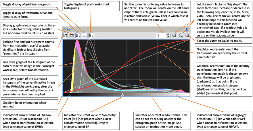
2.2 Multi-function graphical display
A key part of the GHS module interface is the multi-function graphical display. It's main features are described in the diagram below.
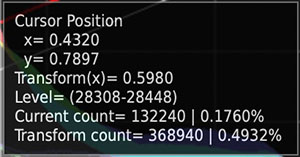
In the GHS interface you can mouse-over the histogram to diplay cross hair cursors. Hover at any point to display histogram and transformation data relating to that point on the graph as shown below. Note: Transform(x), the transformed value of the current cursor x value, is an exact figure. However, Transform count, is the estimated count of pixels falling within the Level range after application of the transformation to the current image.
Important Note about masks: Where the active image has a mask applied, the predicted histogram after application of the current transformation ignores the effect of the mask.
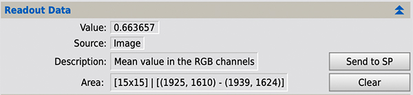
2.3 Readout panel
Data on the readout panel is set by mouse click on either the histogram, the current active image or the real-time preview image. The "Source" data item records whether the data reflects a histogram or an image click.
The readout panel also features two buttons. One will transfer the calculated readout value to the SP parameter (or the BP parameter if Linear transformation is selected). The other button will clear the current readout data.
2.3.1 Histogram readout
Clicking on the multi-function graphical display will set the readout value to the x coordinate of the click point. A vertical indicator line will also be shown on the graph.
2.3.2 Image readout
Clicking on the current active image will set the readout value to a statistic based on a region around the click point. A vertical line will also be shown on the multi-function graphical display indicating the calculated value. The relevant statistic and the region are defined by the settings in the PixInsight Readout Options.
The Readout Options can be set on the Edit>ReadoutOptions menu. The Readout Options dialog is shown below.
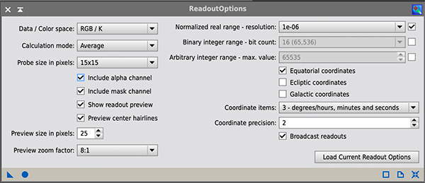
The three parameters of primary relevance to GHS are:
- Calculation mode: this defines the statistic that will be calculated and can be set to Average, Median, Minimum or Maximum.
- Probe size in pixels: this sets the region over which the relevant statistic is calculated from a single pixel up to a 15px x 15px square region. For setting GHS parameters, usually sampling over a larger area will be preferred and hence we suggest setting this parameter to 15x15.
- Broadcast readouts: make sure this is checked so that GHS will be notified if you activate a readout.
For a colour image the statistic is calculated within the specified probe size region over the channels defined by the Mode parameter on the Colour Options panel. The relevant channels are confirmed in the Description on the Readout Data panel.
The readout can be activated by clicking on either the active image or, if available, the real-time preview. It is worth noting that the real-time preview image is a 16 bit integer representation of the active image. Therefore, when clicking on the preview, the standard PixInsight popup readout reflects values calculated on the preview image. By contrast the statistic calculated by GHS is derived from the equivalent point on the actual image and so might differ slightly. When clicking on the active image the GHS and PixInsight calculations should be consistent.
2.4 Control bar
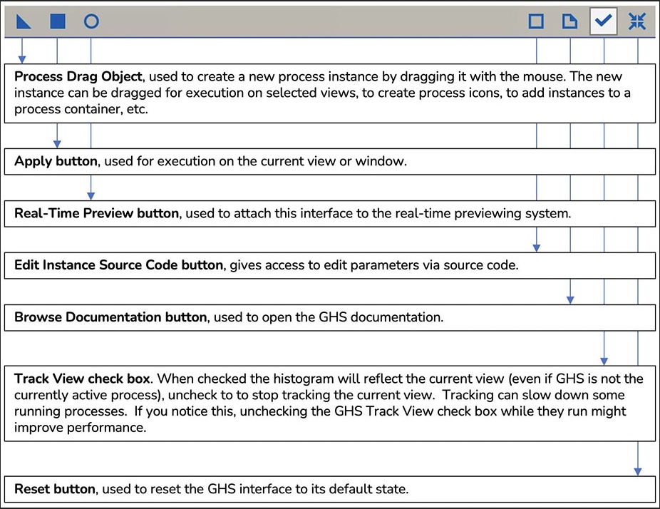
GHS uses a standard PixInsight control bar. The buttons available and their functions are described in the diagram below.
3 Parameters
[hide]
3.1 Mode
Specifies how the transformation is to be applied.
Mode |
Meaning |
Red |
Transformation is applied only to pixel values in the red channel. |
Green |
Transformation is applied only to pixel values in the green channel. |
Blue |
Transformation is applied only to pixel values in the blue channel. |
RGB/K |
Transformation is applied to pixel values in all three channels of a colour image or to the one channel of a greyscale image. |
Lightness |
The image is transformed into the CIE L*a*b* colour space. The transformation is then applied to the CIE L* channel values. The image is then returned to the RGB colour space. |
Saturation |
The CIE L* channel is extracted from the image. The image is then transformed into HSV colour space and the transformation is applied to the Saturation channel. The transformed HSV image is transformed to the CIE L*a*b* space and the L* channel is replaced by the L* channel extracted from the original image. The image is then returned to RGB colour space. |
Colour |
This mode reflects the approach used in the arcsinh process. A weighted average, say z, of the red, green and blue channels is calculated. By default equal weights are used to calculate z (ie a straight average), but see the "Use RGB working space" parameter below. The transformation is applied to z to give T(z). Then each channel is transformed by multiplying by T(z)/z. This can lead to pixel values that exceed 1, the manner in which such pixel values are adjusted is specified by the "Clip type" parameter. |
If GHS is applied to a greyscale image the Colour options, including the Mode, are not relevant. If Track View is enabled and the current active view is greyscale the Colour options are disabled.
3.2 Clip type
Specifies, for a colour stretch, what to do if any channels relating to a specific pixel transform to a value greater than 1.
Clip type |
Meaning |
Clip |
This is the simplest approach. Values greater than 1 are simply truncated to 1. |
Rescale |
The red, green and blue channels are each transformed. The greatest transformed value, say m, is identified (ie, m = Max(Transformed(red), Transformed(green), Transformed(blue))). If m > 1, each of the three transformed channel values is multiplied by the factor (1/m). Note this adjustment factor is calculated on a pixel by pixel basis. This differs from the "Protect highlights" parameter in the ArcsinhStretch process where a single adjustment factor is calculated across the whole image rather than separately by pixel. |
RGBBlend |
The (r, g, b) values are transformed first using the Colour mode to give (r', g', b') say. Then the original (r, g, b) values are transformed using the RGB mode to give (r", g", b"), say. Finally the largest value of k is identified such that k*r'+(1-k)*r"≤ 1; k*g'+(1-k)*g"≤ 1; and k*b'+(1-k)*b"≤ 1. Then the transformed values are calculated as (k*r'+(1-k)*r", k*g'+(1-k)*g", k*b'+(1-k)*b"). |
RescaleGlobal |
RescaleGlobal works in the same way as Rescale except that the maximum value of m is found across all pixels in the image and then all pixel values are reduced by the same factor 1/m. This is the same approach as the "Protect highlights" parameter in the ArcsinhStretch process. |
3.3 Colour blend
When using the colour mode this parameter will blend in a proportion of a standard RGB transformation. This will mute the colour saturation for a strong initial data stretch. A value of 1 is equivalent to a normal colour mode transformation, a value of 0 is equivalent to a normal RGB mode transformation. Values between 0 and 1 give a linear blend between Colour and RGB modes. Note that the blend is applied before checking if any values exceed 1 and require adjustment in line with the "Clip type" parameter. In this sense, using the colour blend slider differs slightly from creating two images, one using the colour mode and the other using the RGB mode, and then blending the two images in, say, PixelMath.
Important note about predicted histogram: when a colour blend value less than 1.0 is set, the predicted histogram shown in the multi-function graphical display does not allow for the RGB blend, it only represents the predicted histogram of the colour mode transformation.
Valid range: [0, 1]
3.4 Use RGB working space
If checked, this parameter instructs the module to use the D50 Luminance Coefficients from the RGB working space of the active image to derive the RGB weighted average for a colour mode transformation. The coefficients can be viewed and amended using the RGBWorkingSpace process. Note that in calculating the weighted average the luminance coefficients are applied to the unadjusted red, green and blue pixel values, ie no gamma adjustment is made. The weighted average is not therefore the same as the CIE Luminance channel, ie the Y channel in CIEXYZ colour space.
If this parameter is left unchecked then equal weighted coefficients will be used.
3.5 Transformation type
Specifies the transformation equations to use. There are four options:
- Generalized hyperbolic.
- Midtone transfer (as used in the HistogramTransformation process).
- Arcsinh (as used in the ArcsinhStretch process).
- Power law (sometimes referred to as a Gamma transformation).
- Linear (equivalent to the shadows, highlights, low and high range parameters of the HistogramTransformation process).
The equations relating to each transformation type are presented in the transformation equations section of this document.
3.6 Invert
If checked, this parameter will cause the inverse form of the transformation equations to be used.
If using the Generalised Hyperbolic, Arcsinh, Midtone transfer or Power law transformations, and the RGB or individual colour channel modes, this allows you to recover your original image subject to mathematical precision, by applying the inverse transformation. Note that, although the GHS transformation is mathematically invertible, the manner in which the transformation is employed in the Lightness, Saturation and Colour modes is not invertible. Hence, while the module will allow you to use the inverted transformation for these modes, this won't necessarily get you back to your original image.
Linear transformations are not necessarily invertible, specifically they are not invertible if BP is greater than zero and/or WP is less than 1.0. Nonetheless, the GHS module will permit inversion with the convention that, if BP is greater than zero the inverse transformation transforms a zero value to the BP value and, if WP is less than 1.0, a value of 1.0 transforms to the WP value.
3.7 Stretch factor (ln(D + 1))
This parameter controls the amount of stretch. If the Stretch factor is set to zero there is no stretch, ie the transformation is the identity transformation.
Note that the value entered is converted for use in the GHS formulae. So, if a value of x is entered for this parameter, the value of D used will be: ex - 1.
Valid range: [0, 20]
3.8 Local intensity (b)
This parameter controls how tightly focused the stretch is around the Symmetry point (SP) by changing the form of the transform itself. For concentrated stretches (such as initial stretches on linear images) a large +ve b factor should be employed to focus a stretch within a histogram peak while de-focusing the stretch away from the histogram peak (such as bright stars). For adjustment of non-linear images, lower or -ve b (and/or lower D) parameters should be employed to distribute contrast and brightness more evenly. Large positive values of 'b' can be thought of as a histogram widener, ie spreading the histogram wider about the focus point, SP. By contrast, lower and -ve values of b tend to shift the histogram to a brighter (or dimmer) position without affecting its width too greatly. As a general rule, the level of b employed will decrease as a stretch sequence nears completion, although larger +ve b values (with small D) can still be employed for precise placement of additional contrast.
Valid range: [-5, 15]
3.9 Symmetry point (SP)
Sets the focus point around which the stretch is applied - contrast will be distributed symmetrically about SP. While 'b' provides the degree of focus of the stretch, SP determines where that focus is applied. SP should generally be placed within a histogram peak so that the stretch will widen and lower the peak by adding the most contrast in the stretch at that point. Pixel values will move away from the SP location.
Valid range: [0, 1]
3.10 Protect shadows (LP)
Sets a value below which the stretch is modified to preserve contrast in the shadows/lowlights. This is done by performing a linear stretch of the data below the 'LP' level by reserving contrast from the rest of the image. Moving the LP level towards the current setting of SP changes both the scope (range) and the amount of this contrast reservation, the net effect is to push the overal stretch to higher brightness levels while keeping the contrast and definition in the background. The amount of contrast reserved for the lowlights is such that the continuity of the stretch is preserved. This parameter must be greater than or equal to 0 and not greater than the Symmetry point.
Valid range: [0, SP]
3.11 Protect highlights (HP)
Sets a value above which the stretch is modified to preserve contrast in the highlights/stars. This is done by performing a linear stretch of the data above the 'HP' level by reserving contrast from the rest of the image. Moving the HP level towards the current setting of SP increases both the scope (range) and the amount of this contrast reservation, the net effect is to push the overal stretch to lower brightness levels while keeping the contrast and definition in the highlights. The amount of contrast reserved for the highlights is such that the continuity of the stretch is preserved. This parameter must be less than or equal to 1 and not less than the Symmetry point.
Valid range: [SP, 1]
3.12 Blackpoint (BP)
Sets the Blackpoint for a linear stretch of the image. Note that any pixel with values less than the Blackpoint input will be clipped and the data lost. Contrast gained by performing the linear stretch will be evenly distributed over the image, which will be dimmed. Pixels with values less than the Blackpoint will appear black and have 0 value. Updating this parameter will automatically update the low clipping proportion. Setting this parameter to a value less than 0 will extend the dynamic range at the low end.
Valid range: [-1, WP)
3.13 Whitepoint (WP)
Sets the Whitepoint for a linear stretch of the image. Note that any pixel with value greater than the Whitepoint input will be clipped and the data lost. Contrast gained by performing the linear stretch will be evenly distributed over the image, which will be brightened. Pixels with values greater than the Whitepoint will appear white and have a value of 1.0. Updating this parameter will automatically update the high clipping proportion. Setting this parameter to a value greater than 1 will extend the dynamic range at the high end.
Valid range: (BP, 2]
4 Setting parameters
[hide]
4.1 Methods of setting numerical parameters
Parameter |
Methods of setting value |
Stretch factor |
Input text box |
Local intensity |
Input text box |
Symetry point |
Input text box |
Protect shadows |
Input text box |
Protect highlights |
Input text box |
Blackpoint |
Input text box |
Whitepoint |
Input text box |
4.2 Use of Fine adjustment slider
The Fine adjustment slider can be used to adjust any of: D, b, SP, LP, HP, BP, WP, LCP or HCP. For all parameters other than D and b, its sensitivity can be adjusted with the "Use highest sensitivity" checkbox. When stretching linear data it will normally be appropriate to use the highest sensitivity which will make adjustments in the 6th decimal place of the relevant parameter. For subsequent stretches lowering the sensitivity may be appropriate, unchecking the checkbox will make adjustments in the 4th decimal place. For the D and b parameters the Fine adjustment slider will make adjustments at the 3rd decimal place.
4.3 Low and high clip settings
When performing a linear stretch it is possible to set the Blackpoint to a value that results in some currently non-zero pixels being set to zero. Likewise the Whitepoint may be set so that some non-unity pixels are set to a value of 1.0. This is referred to as low or high clipping respectively.
When the Blackpoint parameter is adjusted, the proportion of pixels that would be low clipped if that Blackpoint were applied to the current active image is automatically calculated and displayed in the Low clip (LCP) data item. Similarly for the Whitepoint and High clip data item.
The reverse process can also be applied. If a clipping proportion is set as the Low clip data item, GHS will automatically calculated the highest value of Blackpoint such that the proportion of clipped pixels in any of the relevant channels (as defined by the Mode parameter in the Colour options panel) does not exceed the specified value. Similarly for the High clip data item and Whitepoint.
5 Transformation equations
[hide]
5.1 Linear
The linear transformation type is defined by the folowing:
Range |
Transformation |
x ≤ Blackpoint |
y = 0.0 |
Blackpoint < x < Whitepoint |
y = ( x - Blackpoint )/( Whitepoint - Blackpoint ) |
x ≥ Whitepoint |
y = 1.0 |
The inverse linear transformation is defined as follows:
y = Blackpoint + x.( Whitepoint - Blackpoint )
subject to minimum 0.0, and maximum 1.0.
5.2 Non-linear
5.2.1 Definition of variables
D = e(Stretch factor) - 1
b = Local intensity
SP = Symmetry point
LP = Protect shadows
HP = Protect highlights
m = 0.5 / (D + 1)
5.2.2 Base transformation equations
The base transformation for each transformation type is defined by T : x → T(x) in the following table. The table also shows the first derivative of T, denoted T', as this is needed to build the full transformation.
Transformation type |
Subtype |
Conditions |
T(x) |
T'(x) |
Generalised hyperbolic |
Logarithmic |
b = -1 |
ln( 1 + D.x ) |
D/( 1 + D.x ) |
Generalised hyperbolic |
Integral |
b < 0, b ≠ -1 |
(1 - (1 - b.D.x)((b + 1)/b))/(D.(b + 1)) |
( 1 - b.D.x )(1/b) |
Generalised hyperbolic |
Exponential |
b = 0 |
1 - e-D.x |
D.e-D.x |
Generalised hyperbolic |
Harmonic |
b = 1 |
1 - ( 1 + D.x )-1 |
D.( 1 + D.x )-2 |
Generalised hyperbolic |
Hyperbolic |
b > 0, b ≠ 1 |
1 - ( 1 + b.D.x )(-1/b) |
D.(1 + b.D.x)(-(1+b)/b) |
Midtone transfer |
(m - 1).x / ( (2m - 1).x - m ) |
m.(1 - m).((2m - 1).x - m)-2 |
||
Arcsinh |
arcsinh(D.x) = ln( D.x + √( D2.x2 + 1 ) ) |
D/(√(D2.x2 + 1)) |
||
Power law |
1 - (1 - x)1 + D |
(1 + D).(1 - x)D |
5.2.3 Building the full transformation
We describe below how the full transformations are built from the base equations. We assume that: 0 < LP < SP < HP < 1, if any of these inequalities are infact equalities the adjustment required to what follows should be evident. We also assume D > 0, if D = 0 the transformation is simply the identity transformation.
- The maximum gradient for the base equations occurs at x=0. This point defines the point of maximum intensity and we want that to occur at x = SP. So we transform the equation by defining:
T3(x) = T(x-SP).
This broadly defines the transformation for the range SP ≤ x < HP although it will need to be normalised as described later below. - The transformation for LP ≤ x < SP is defined by symmetry as follows:
T2(x) = -T(SP-x).
This, in effect, is equivalent to rotating the graph above SP through 180° around the point (SP, 0) - hence the name, Symmetry point. - For the range 0.0 ≤ x < LP we want a linear transformation so we calculate the gradient of T2 at LP, ie T2'(LP), where the prime represents the first derivative. We also want the line to pass through the point (LP, T2(LP)). So we define:
T1(x) = T2'(LP) * (x - LP) + T2(LP) - Similarly for the range HP ≤ x ≤ 1.0, we calculate a linear transformation as follows:
T4(x) = T3'(HP) * (x - HP) + T3(HP) - Finally we want the transformed values to run from 0.0 to 1.0 so we need to normalise. We define:
NormTi(x) = (Ti(x) - T1(0))/(T4(1) - T1(0)), for i = 1, 2, 3, 4
We then define the full transformation: NormT: x → NormT(x), as follows:
Range |
NormT(x) |
0 ≤ x < LP |
NormT1(x) |
LP ≤ x < SP |
NormT2(x) |
SP ≤ x < HP |
NormT3(x) |
HP ≤ x ≤ 1 |
NormT4(x) |
5.2.4 Inverse transformation equations
The base inverse transformation for each transformation type is defined by InvT : x → InvT(x) in the following table.
Transformation type |
Subtype |
Conditions |
InvT(x) |
Generalised hyperbolic |
Logarithmic |
b = -1 |
(ex - 1)/D |
Generalised hyperbolic |
Integral |
b < 0, b ≠ -1 |
(1 - (1 - (b+1).D.x)(b/(b+1)))/(D.b) |
Generalised hyperbolic |
Exponential |
b = 0 |
-ln(1 - x)/D |
Generalised hyperbolic |
Harmonic |
b = 1 |
x/(D.(1 - x)) |
Generalised hyperbolic |
Hyperbolic |
b > 0, b ≠ 1 |
((1 - x)-b - 1)/(b.D) |
Midtone transfer |
m.x / ( (2m - 1).x - (m - 1) ) |
||
Arcsinh |
sinh(x)/D = (ex - e-x)/(2D) |
||
Power law |
1 - (1 - x)1/(1 + D) |
Then we can define the full inverse transformation InvNormT: x -> InvNormT(x), as follows:
Range |
InvNormT(x) |
0 ≤ x < NormT(LP) |
LP + (x' - T2(LP))/T2'(LP) |
NormT(LP) ≤ x < NormT(SP) |
SP - InvT(-x') |
NormT(SP) ≤ x < NormT(HP) |
SP + InvT(x') |
NormT(HP) ≤ x ≤ 1 |
HP + (x' - T3(HP))/T3'(HP) |
where
x' = T1(0) + x.(T4(1) - T1(0))
5.3 Note on precision
For the sake of accuracy, all intermediate calculations in GHS are performed in 64-bit floating point format (i.e. using the double C++ data type).
6 Tips on usage
[hide]
Much has been written and recorded on-line and we have no ambitions to match that resource here. This section provides some brief suggestions on use of GHS that we hope will help get new users started.
6.1 Initial stretch of linear data
Many of the tools available to move your data from linear to non-linear are designed to make all, or at least substntially all, the process in one go. This inevitably involves some compromises. GHS is designed to provide much greater control and as such it will typically take two or more stretches to get to a non-linear image ready for further processing. This section describes the first step in this process.
- When stretching data from its linear state it will be useful to use the "big zoom" button (the magnifying glass with "+" on it) on the multifunction graphical display. This will help to reveal the histogram which will typically be right over on the left hand side of the graph.
- We recommend using the Generalised Hyperbolic transformation type as this gives the greatest control over the "shape" of the transformation.
- The maximum focus of the stretch should normally be set close to the point where the background gives way to data that is of interest. This can be found to a first approximation by clicking on the image at a point where the dimmest data you wish to reveal is located. (You will need the STF activated on your image to be able to see this).
- The resulting value will be displayed in the readout panel. You can see where in the histogram this point is from the gold vertical indicator line on the multifunction graphical display. Typically for a galaxy this will be to the right of the histogram peak; for images where nebulosity covers most of the image the point will be closer to the histogram peak and may even be slightly left of the peak.
- This value can be transferred to the Symmetry point parameter, which is the point where the maximum stretch intensity will be focused, by pressing the Send to SP button.
- Having set the initial SP value, you will want the stretch to be strongly focused in this region so set a high value of Local intensity parameter, perhaps around 10.
- Now reset the multifunction graphical display zoom to 1x by pressing the right-most magnifying glass button. This will allow you to see the full histogram graph as you increase the Stretch factor. You want to increase this parameter until the histogram peak moves to a value of around 0.2- 0.25.
- Now for the fine tuning, remove the STF from your image and press the circle at the bottom left of the GHS interface dialog. This will reveal the real-time preview. You can adjust the value of SP - be careful it is very sensitive, so use the Fine adjustment slider with "Use highest sensitivity" checked.
- Don't worry that the image is looking rather "flat" at this stage. For this stretch you are using your contrast "budget" to separate useful data from the background, so the rest of the image will be flat. Juggle D, b and SP to find a combination you are happy with. You wont need LP at this stage and you are unlikely to need HP as the nature of the GHS transformation is such that the brighter stars will be quite well protected from burn-out by the high Local intensity (b) parameter.
- When you are happy, apply the transformation by hitting the square button at the bottom left of the GHS interface dialog.
6.2 Preserving colour and saturation in the initial stretch
When stretching linear colour data, it often happens that the resulting image is somewhat lacking in colour saturation. This is a direct consequence of the "shape" of the transformation and how it is applied. Colour saturation at a given pixel is defined by the proportional difference between the brightest of the RGB channels and the dimmest. The initial stretch will tend to stretch lower values proportionally more than higher values. So, when the transformation is applied this proportional difference, ie the saturation, tends to be reduced. This section discusses a possible way to mitigate this.
- The Colour mode, found on the Colour options panel, will maintain the colour saturation of your image. How this mode works is described in the Colour mode description above but essentially it ensures that, for each pixel, the same proportionate stretch is applied to each channel. When appraising your initial stretch, try choosing the Colour mode rather than RGB and you will see the difference.
- Sometimes the Colour mode can result in an image which is overly saturated for your taste. The Colour blend slider will allow you to mute the effect by blending some RGB mode stretch back into the resulting image.
- Unfortunately there are no free lunches! A drawback of the Colour mode is that it can result in some clipping of data in bright channels. The way the clipping is dealt with is defined by the Clip type parameter. It will generally be the core of bright stars that will be affected, so zoom into a few and try different Clip types - RGBBlend often works quite well.
- It is worth being aware that the potential for data clipping means the Colour mode stretch is not invertible. If it is important to you to be able to analytically invert the stretch (as distinct from simply clicking the PixInsight "undo" button) then you should not use the Colour mode.
6.3 Adding contrast to a non-linear image
Once your pixel data is non-linear, initially it will likely be lacking in contrast (as noted above). It is therefore likely that you will want to add contrast in some key ranges to improve the visual presentation of those parts of the image you want to emphasise. This section gives some pointers for this process.
- Make sure you don't have a STF applied to your image.
- Examine the image and decide where there are some flat-looking areas that are important to you and you want to emphasise.
- Click in such a target area of the image to obtain a pixel value readout in that area. For this we suggest you set the readout probe size to 15x15 and the readout/calculation mode to mean. How this is done is explained above.
- The readout value will be highlighted on the multifunction graphical display with a gold indicator line. Note that this value may well coincide with an area where the Histogram has a slight "hump" indicating a bunching of pixels at a particular intensity level. Indeed looking for Histogram humps is another way to identify value ranges that could use an injection of contrast.
- Displaying the Histogram graph on a Log scale can be very helpful at this point. You will now be focusing less on background pixels (generally the histogram peak) so the Log display will allow a better appraisal of contrast distribution in the lower to mid pixel counts. It will also help to see how the stars (generally over to the right of the histogram graph) would be affected by any proposed transformation.
- Click on the Send to SP button to transfer the readout value to the Symmetry point parameter.
- It is likely that you will want to spread the contrast over a range of intensity values so a mid-range Local intensity value might be appropriate to achieve what is needed. Perhaps a value in the range 3 - 5 may be a good starting point.
- Now open up the real-time preview and move the Stretch factor slider until you start to see the effect you want. You will probably need to work with the Local intensity (b) slider and the Symmetry point (SP) as well. Adjusting the latter can be done using the Fine adjustment slider but you probably will want to un-check "Use highest sensitivity".
- There is a danger that these subsequent stretches can start to affect your brighter stars. Moving the Protect highlights (HP) slider can help to preserve these.
- There is also a danger that the background can start to get too dark. The Protect shadows (LP) slider can be used to "push" the histogram back over to the right and thereby preserve the shadow brightness.
6.4 Darkening the background by setting the blackpoint
GHS allows a blackpoint to be set such that all pixel values lower than the blackpoint will be set to zero and contrast is redistributed linearly across the rest of the image. To achieve this select the Linear option under Transformation type. This approach typically leads to some pixels being clipped to zero and hence to loss of data. This is not a problem per se but it may be interesting to note that GHS can be used to do something very similar but with no data clipping.
- Select the Generalised Hyperbolic transformation type (not Linear).
- Set the Symmetry point (SP) to a value below which you want the transformation to set pixel values at or close to zero.
- Set the Protect highlights (HP) parameter equal to SP.
- Leave the Protect shadows (LP) parameter at zero.
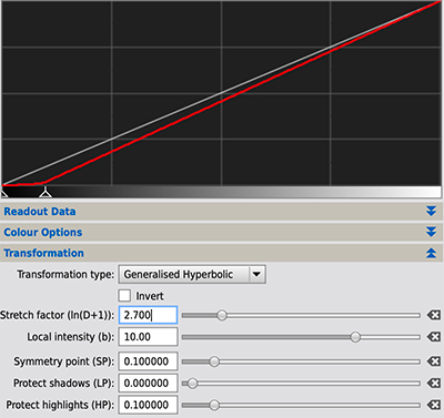
- Set Local intensity (b) to a high value, eg 10.
- Move the Stretch factor parameter slider to create a transformation shape similar to that depicted below.
6.5 Luminance stretch
It is common procedure to process colour data separately from the luminance data and for these to be combined at a later point in the non-linear workflow.
It can be difficult in this process to ensure the luminance channel has been stretched exactly as desired. Although experience helps, the actual result of the combination wont be entirely clear until the images have been combined. Adjusting the stretch of the Luminance normally requires restretching and recombining until you are happy.
GHS provides an alternative interactive approach, described below, using the Lightness mode in the Colour options panel.
- Use your experience to get the Luminance channel as close to what you want as possible.
- Add the Luminance channel to your Chrominance image in the normal way, eg using the LRGBCombination process.
- Select the Lightness mode in the Colour options panel.
- Open up the real-time preview and use the GHS parameters to adjust the "Luminance" as desired.
(Note that, although we often refer to the Luminance channel, infact the channel added using the LRGBComination process is a Lightness (L*) channel in CIEL*a*b* colour space.)
6.6 Using GHS with star removal software
The removal of stars has become an integral part of the workflow for many astrophotographers. In our experience, the most common AI based star removal tools in current use do not deal well with identifying brighter stars that have been stretched using GHS. We therefore recommend starless images are generated by one of two methods:
- If the star removal tool has an option to run on linear data then use this and remove stars before stretching your images to non-linear. The stars image and the starless image can then be stretched separately to non-linear.
- Otherwise, make a moderate stretch of your data - if using the Generalised Hyperbolic transformation type ensure you leave the Local intensity (b) parameter at zero (this will help the star removal software to recognise your stars). If you have a colour image make sure to choose RGB mode in the Colour options panel not Colour mode (the Colour mode can result in clipping and hence is not invertible). Next remove the stars using your preferred star removal tool. Finally check the Inverse checkbox in GHS but leave all other parameters exactly as for your initial moderate stretch and apply this to the starless image and the extracted stars image to return these to their linear state.
7 Disclaimer and Licence Information
[hide]
The GeneralizedHyperbolicStretch process module is based on software from the PixInsight project, developed by Pleiades Astrophoto and its contributors (https://pixinsight.com/).
This program is free software: you can redistribute it and/or modify it under the terms of the GNU General Public License as published by the Free Software Foundation, version 3 of the License. This program is distributed in the hope that it will be useful, but WITHOUT ANY WARRANTY; without even the implied warranty of MERCHANTABILITY or FITNESS FOR A PARTICULAR PURPOSE. See the GNU General Public License for more details. You should have received a copy of the GNU General Public License along with your PixInsight installation. If not, see http://www.gnu.org/licenses/.
Copyright © Mike Cranfield 2022, 2023